Quantcast
Channel: Guy on Simulink
Viewing all 159 articles
Browse latest View live

Offload work from your computer by running simulations on a remote cluster

$
0
0

Recently, I noticed that when I right-click on a MATLAB script in the Current Folder Browser, there is an option to run the script as a batch job.

Run Script as Batch Job

As you can guess, the first thing that when through my mind is: I want the same thing to simulate a Simulink model!

Let's see what I came up with.

Background

For those not familiar with the Parallel Computing Toolbox, you might be wondering: What is a batch job?

As explained here, the batch command can launch a new MATLAB session in the background and run a script or function there. You can then continue to work in your current MATLAB session without the need to wait for the script to complete.

Run Script as Batch Job

In addition to the Parallel Computing Toolbox, if you also have access to a MATLAB Distributed Computing Server, the batch job can be executed on a remote cluster, leaving all the computing power of your machine to perform other tasks.

Run Script as Batch Job

My solution

I don't think it is possible to add entries in right-click menu of the Current Folder Browser, so I decided to use an sl_customization file to add a new Simulate as Batch Job entry in the Simulation menu of the Simulink editor.

Simulink as Batch Job menu

I associated the menu entry with the following function:

Simulink as Batch Job code

Let's see what it does and why.

Files Dependencies

One of the first things you will notice if you try simulating models on a remote cluster is that your job usually depends on many files.

If your remote cluster has access to the same file system as your local MATLAB, I recommend taking advantage of that, it will make your life significantly easier. Just adding the same path to the batch job should help avoiding any missing files dependencies.

In my case, I have a Windows workstation, the cluster operating system is Linux, and they do not share a common file system. This means that I need to attach files to the job. The batch command has the capability to analyze the dependencies of your code and automatically attach files to the job. However this functionality does not work very well with Simulink models.

Because of that, the first things I do is call dependencies.fileDependencyAnalysis to find all the files necessary to simulate my model. In the example I am working with, it finds an initialization script used in the model preLoadFcn callback, the model itself, and a referenced model.

File dependencies

Getting the data at the right place

As I explained in a previous post, it can sometimes be tricky to get Simulink to see the data it needs when used through the Parallel Computing Toolbox. One thing that helps is to force the data needed by the model to be in the base workspace by using evalin or assignin.

For a model to work with my menu entry, the model needs to create all the data it needs itself, and place it in the base workspace. The way I recommend to do that is through the model preLoadFcn callback.

preLoadFcn

Creating the job

I am now ready to create my batch job. I pass to batch the cluster where to run, a handle to the sim command, inform it that sim will return one variable, and takes the model name as input. I tell it to not try to analyze my files and automatically attach them. Instead, I pass it the list of files mentioned above. Finally, I tell it to not try to cd to the current directory of my Windows workstation... since it does not exist on the Linux cluster.
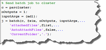
Creating the batch job

Finally, I assign the batch job object in my local base workspace.
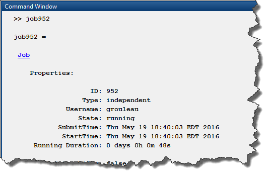
Batch job object

Once the job is completed, use the fetchOutputs method to retrieve the simulation outputs

A few tips...

The first time you will try simulating your model, you will very likely run into various issues. Since the parallel worker runs in the background, it can sometimes feel like debugging while being blindfolded. Here are a few tricks I like to use:

  • To understand what is going wrong on a worker, try displaying information at the worker command prompt. You will be able to visualize it when the job completes using the diary function. Functions like pwd, whos and dir are usually good starting points.
  • If your Simulink model errors out, try placing the sim command inside a try-catch statement and return the error as output instead of the simulation log. Sometimes the error message contains many levels and getting the full error object should help.
  • To debug issues interactively on workers, try using using pctRunOnAll. Similarly to the diary tip above, try running commands like pwd, whos, dir, etc, on workers to diagnose possible problems.
  • Now it's your turn

    We are currently working on features to facilitate this workflow for future releases, but for the current release, I hope this blog post will help you taking advantage of your cluster to run simulations.

    I do not guarantee that my sl_customization will work for all models, but I believe it will work with many setups. If not, I hope this can help as a starting point for you to simulate models on remote clusters.

    Give it a try and let us know how it goes by leaving a comment here


Three-Way Model Merge and Git

$
0
0

In R2016a, a new Three-Way Model Merge functionality got introduced. You can find a clear description of this feature in the following documentation pages:

In those documentation pages, the workflow always begins with right-click on the conflicted model file and select View Conflicts.

Conflicted file

In this blog post, I will try to provide a bit of additional information to complement the workflow described in the above links.

Creating a Conflict

I created a simple project under Git source control. I could have used GitHub, but I decided to use a Git server we have at MathWorks. At the Git command-line, I cloned two identical repositories:

Git Clone

two Projects

In the first repository, I make some modifications to the model. I go in the Modified Files view of the Simulink Project, commit the modified files and push the changes to the remote repository

commit and Push

I close the first project, navigate to the second repository, open the Simulink Project there, and modify the model in a different way.

Resolving the Conflict

Before trying to commit and push changes as done in the first repository, it is always a good idea to click the Fetch button to get the latest from the remote repository. Once this is done, you can see if the remote master branch has new submissions. If it does, you want to merge with it before pushing your changes.

Merge

Because of the conflict, you will receive this error:

Merge Error

If you go back to Simulink Project, the conflicting files will look like:

Git Conflict

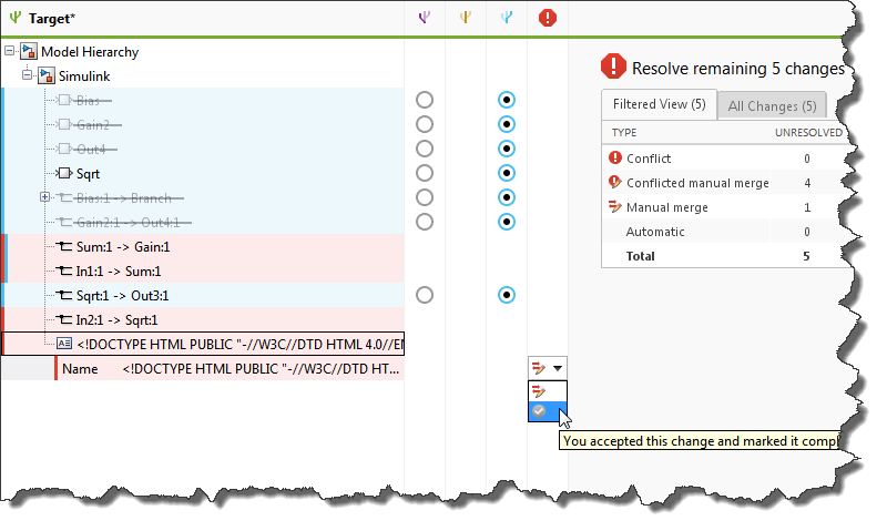
Right click on the file and select View Conflicts to launch the Three-Way Model Merge tool. You will then be able to see:

  • The original model
  • The latest model in repository 1
  • The latest model in repository 2
  • A target model automatically generated by Simulink, attempting to do its best guess at merging the three previous models.

Three-Way Model Merge

In the bottom left section of the Three -Way Model Merge, for each block and signal, you can select which version you want to be merged in the target model. For conflicts that cannot be automatically merged, you can manually fix them in the target model and individually mark them as resolved.

Since the versions from repository 1, repository 2 and the target model can all be opened at the same time, this makes the manual resolution of conflicts quite easy.

Zoom on model merge

Once you are satisfied with the target model, click the Accept & Close button:

Accept and Close

You will then be able to Commit the modified files and push the changes to the repository. If you click the Manage Branches button, you should see how the project got branched and merged back.

branch evolution

One more tip...

In most cases, this kind of merging challenges happen within the context of a project under source control. However if you just want to launch the tool without any project or source control involved, you can use the following syntax:

slxmlcomp.slMerge(baseFile, mineFile, theirsFile, targetFile);

where the 4 inputs are four model files.

Now it's your turn

How do you manage branching? Give a try at the Three-Way Model Merge and let us know what you think by leaving a comment here.

Another Good Reason to Log Simulation Data in Dataset Format

$
0
0

Today I am happy to welcome guest blogger Mariano Lizarraga Fernandez. A few days ago, Mariano came to me looking for help understanding a Simulink behavior that a user was not able to explain. Once we figured it out, we thought it would be good to share with you.

Introduction

In R2015b we introduced the possibility to save states and outputs in Dataset format. In R2016a, these capabilities were further extended to log units, and for large amounts of data, to be able to log data directly to a MAT-file. I could list tons of reasons why the Dataset format is more convenient than other options, but for today what I want to share is an example where the dataset format could have helped avoiding lots of confusion.

Serializing Data from frames

I was recently helping a customer who was logging frames-based signals with a variable-step solver and saving it to the workspace. If the frame-based data was serialized (i.e each frame was stacked on to the last one creating a n x 1 vector) and plotted, the data showed what looked like every once in a while a frame was repeated, causing discontinuities every given number of frames.

Take for instance the following model, which uses a variable-step discrete solver and contains two different sample times. The model is configured to save outputs in the Structure with Time format:

Frames Example 1

Serializing and plotting the outport's 'Out1' data, one can see the repeated frames:

Frames output

The Structure with Time documentation explains that it contains a single vector of the simulation times. This has two implications:

  1. The time vector contains the union of all sample time vectors used in the model.
  2. For the signal values to be consistent with the time vector, its value must be logged at every sample time contained in the time vector.

Using Dataset to Log Data at Different Sample Rates

To better understand these implications, let's get rid of the frame and consider the following model which saves 3 ramp signals:

Simple Model

Let us now run the simulation and log the output of all three outports in two different formats: Structure With Time and Dataset. To see the effect of the single time vector of the structure with time format, I like to plot the data using the stem function.

Simple model output

With the Dataset format, each signal is a timeseries object with its own sample time. Whereas for the Structure with Time, since there is only a single time vector, data has to be recorded for all outputs at every sample time.

Now its Your Turn

If you are logging simulation data using Structure with Time, I recommend using the Dataset format instead as it is more flexible and gives you independent time vectors. This format also allows you to log units information, you can log directly to a MAT-file, and can even log multiple values for a single time step, which is useful inside iterator subsystems.

Give it a try and let us know what you think by leaving a comment here.

It’s Time for Real-Time!

$
0
0

Today, I am happy to welcome guest blogger Sarah Dagen, from MathWorks Consulting Services to talk about real-time simulation and testing.

Why Real-Time?

Working in MathWorks consulting services, one of my favorite things is helping customers with real-time simulation and testing. Since many aspects of this technology have not been discussed before on this blog, I am going to walk through a design task that leverages many of the benefits of Simulink Real-Time and real-time simulation and testing.

Design Task

Let’s begin with an example problem: Guy and I decide that we really need to develop a device that will fetch us beverages from the kitchen, saving us the enormous exertion of having to stand up and walk to get it ourselves.

The Robot

At a very high level, the system comprises 2 components:

  1. A physical device that will walk (or roll, or fly) to the kitchen, get the requested beverage, and bring it to us;
  2. An embedded controller that will control the actions of the physical device.

Since Guy is a mechanical engineer and much better at this than me, I’ve asked him to develop the physical device (the “plant”, in control design speak). I’m going to develop the controller.

Desktop Simulation

Not surprisingly, Guy soon sends me a simulation model of his robot. We want to make sure the physical device and the controller interact properly before we invest in the production of the final system. Meanwhile, I’ve developed a control algorithm in a model.

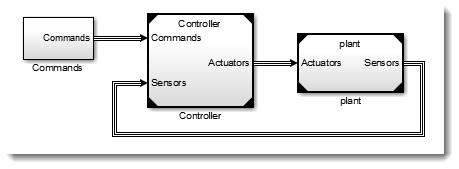
Using model referencing, we connect the plant and controller models to simulate the entire system.

Simulating the Robot

After a few rounds of iterating on our designs, we have a design that we think could work.

So what do we do next?

Let’s Real-Time!

To simulate our models in real time, we will be using Simulink Real-Time. With Simulink Real-Time, in one click C code is generated for the model, downloaded to a dedicated system, and executed in real-time. Once the executable is running on the target, we can perform automated or interactive testing and create instruments for monitoring and controlling the real-time application.

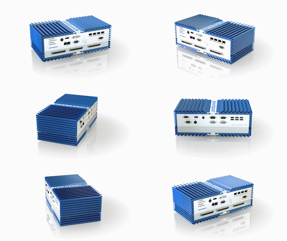
As dedicated target computer hardware, we will use Speedgoat mobile real-time target machines.

Speedgoat target machine

Wondering what Speedgoat is? Speedgoat makes a range of real-time target computers and offers a huge array of hardware I/O connectivity modules. Speedgoat target computers are specially designed and optimized to work seamlessly with Simulink Real-Time.

Now let's talk a bit about our setup. When we talk about real-time simulation and testing, there are 3 basic configurations:

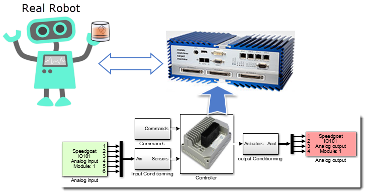
  • Rapid prototyping: the controller is simulated on a real-time target computer, and the real physical plant is connected to it.
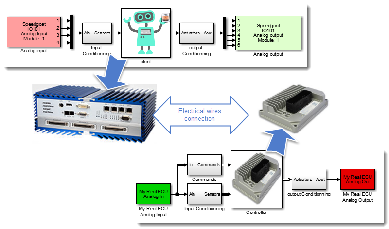
  • Hardware-in-the-loop: the plant is simulated on a real-time target computer, and the real embedded controller hardware is connected to it.
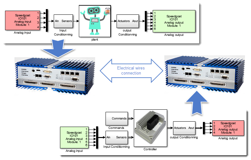
  • All simulation: the plant is simulated on one real-time target computer, and the controller is simulated on a separate real-time target computer, with electrical connections between the two.

Let's see how we apply each of those to our project.

All Simulation

Guy is working on building the physical robot, and I’ve chosen an embedded target hardware for the controller. We have agreed on the electrical interfaces for sensor feedback and control signals between the controller and the physical robot. Before we have received all the mechanical and electrical parts we will need, we’d like to continue to refine our designs.

For the all simulation setup, we have two real-time target computers from Speedgoat. We decided on the mobile real-time target machines because we want to be able perform field testing with our simulations and the rugged mobile design is great for this. Also, they are just straight-up good-looking. Each of the target machines has an analog input/output card which we have chosen because it emulates the electrical characteristics of the real hardware we will use in our beverage-fetching robot. I add the I/O connections to the controller and plant models to for the electrical interfaces.

Here’s an image showing the setup of plant and controller each on real-time simulation target computers:

All real time simulation

Our testing with this real-time configuration reveals that we haven’t properly converted the electrical signals into engineering units – glad we found this out now! We fix the errors and continue with successful testing.

Rapid Control Prototyping

Guy has finished building the first physical robot before my controller hardware has even been shipped. We are both eager to continue development, and now we can test my controller design to see if it can actually control the position of Guy’s mechanical creation.

For this configuration, we replace the Speedgoat target hardware that was simulating the plant with the real physical robot. He doesn’t have an embedded controller yet, so we will use the second Speedgoat target computer as the controller. We build some test harnesses and wire up the I/O connections between the robot and the Speedgoat target computer.

Here’s an image showing this setup:

All real time simulation

Thanks to all of the up-front simulation and testing we’ve already done, Guy and I find that our initial tests trying to control the robot’s position are fairly successful. The control seems to be a bit sluggish, though, and I think that I can improve the algorithm after seeing how it behaved with the real physical device. And since I don’t have to go through the entire embedded code generation process, I am able to quickly make changes to the controls and immediately test the performance. Simulink Real-Time allows me to easily tune parameters in real-time, so I can tweak my controller without having to regenerate any code!

Hardware-in-the-Loop

My controller hardware finally arrives. With a refined control algorithm design ready to go, I generate embedded code and deploy to my new production target.

I call Guy and let him know that it’s time to test my real controller with his robot – but Guy has his own opinions on the matter. He’s not ready to let me endanger his robot masterpiece until I demonstrate to him that there are no issues with the controller deployment.

No problem – I can use a Speedgoat target computer and Simulink Real-Time to simulate the physical robot and connect it to my embedded controller and use hardware-in-the-loop (HIL) simulation to test out the controller. I create a large test suite, including some very aggressive test cases to make sure the control design is robust and failure-tolerant (there are delicious beverages at stake!).

Here's the HIL simulation setup:

Hardware in the loop

Vindicating Guy’s insistence on HIL testing, we discover that a certain combination of faulty sensor feedback signals can cause the controller to command the robot to an unstable position, which our plant model shows could result in the robot spilling the beverage on itself – not good for our beverages, and definitely not good for the robot! I add additional safety logic for such cases and deploy the updates to the controller.

After running through HIL testing, I am pleased with my controller’s performance, and confident that the system will be able to handle aggressive field testing with the real robot.

And finally…

The next day, Guy brings over the robot and we integrate the embedded controller. With a high level of confidence in our well-tested system, we proudly sit back and wait for our drinks to arrive.

Guy and Sarah having a drink

Now it’s your turn…

Do you use real-time simulation and testing in your design processes? Would you like to read more about using Simulink Real-Time? Leave a comment below!

Tips for dealing with Libraries

$
0
0

Today I will share a simple trick that might save you some time if you are dealing with large Simulink models componentized using libraries.

Long Time to Save

Earlier this week, I received a large model made of multiple subsystems stored in a library file. I had to do some modifications to the library. When I was done with my modifications, I clicked on the Save button, it took significantly longer than I expected, more than a minute.

Curious, I decided to profile the saving operation to try understanding what was happening:

Starting the MATLAB Profiler

Here are the results:

Profiler results

The Explanation

When I saw that most of the time was spent in a function called "generateSVG", I knew exactly what was happening.

As described in the documentation page Add Libraries to the Library Browser, if you want your library file to appear in the Simulink Library Browser, you need to enable the EnableLBRepository property of the library.

Enabling Library Browser Repository

When this option is enabled, Simulink will save an image file for each block to be displayed in the Library Browser. This image is in scalable vector graphics format (SVG). You do not see those image files, but they are inside the SLX library file. As far as I understand, this is done to speed up the opening of the Library Browser.

Sure enough, disabling this option made the time to save the library pass from over a minute to just a few seconds.

Disabled Library Browser Repository

Conclusion

Based on that, I recommend turning this flag on or off depending on your workflow. When you are in editing mode and you modify and save the library often, disable EnableLBRepository. When your library is ready to be released and deployed to other users who will access it from the Library Browser, enable EnableLBRepository.

A few more tips...

While we are talking about speeding up workflows, here is another trick I like. In my startup.m, I like to add the following two lines:

Speeding load

By default, Simulink and the Library Browser are loaded in memory only the first time you simulate or open a model. Since I always use Simulink, I prefer having the loading done as soon as MATLAB launches.

Now it's your turn

Do you have other tips or tricks like those? Share them with us by leaving a comment below.

In Libraries, Code or Model Reusability? That is the Question.

$
0
0

This week, Mariano Lizarraga Fernandez is back as guest blogger with a new interesting topic: Model Reusability versus Code Reusability.

Introduction

Every now and then those of us who work in technical support at Mathworks hear variants of the question: "Why is the code generated for my library subsystem not being reused in all the places that it should?"

In this post I will try to explain a concept that I recently discussed with colleagues: Model Reusability vs. Code Reusability.

Model Reusability

Simulink Libraries is one of multiple options you have to implement model componetization. The core idea, akin to traditional programming languages, is that you build a modelling construct that you wish to reuse in multiple places. But, as opposed to traditional programming languages, with Simulink libraries, you get plenty of freedom on how you can use this library block. You can use it under different sample rates, the inputs can be of any data type, provided the building blocks support it, and these inputs can even vary in dimensions from call site to call site.

Take for instance the following subsystem which tries to solve a common pattern encountered in embedded systems: protect from division by zero.

Simulink Library

If I save this subsystem in a library, it can be used in a model, under different conditions, with no change necessary. For example, in the following model I use the subsystem with different data types and dimensions:

Simulink Library reused

If you do this, you will realize that for code generation, in some cases, even if you specify that you want a reusable function, as shown above, you might not get a reusable function:

Simulink Library not reused

So the flexibility that you gain by model reusability, comes with the tradeoff that different functions can be generated for each use of the library subsystems.

Code Reuse

If code reuse is the main concern, then one thing that can be done to improve code reusability is to "tighten" the interfaces of the library. By specifying the data type and dimension on the library inports to be single and 1 respectively, we sacrifice model reusability to improve code reusability. Doing this requires that the above model be modified as follows:

Code reuse

Note how several more blocks had to be added to the model to allow this tightening of the library interface. Nevertheless, this results in a single function with three call sites in the generated code:

Code reuse

Model Checksum

For those cases when you can not determine why your subsystem is not resulting in a reusable function, Simulink offers an API to compute an atomic subsystem's checksum. This checksum gives you access to multiple fields that can help you determine why your subsystem code is not being reused.

If we were to compute the checksum for the first model shown in this post, we would see that the checksums for the ZP_1 and ZP_2 subsystems are different, resulting in code not being reused. You can scroll over the checksums' fields to locate the differences in these, and gain some insight into the reason, in this case, different data types.

Code reuse

Finally, be aware that Checksum is not the only condition to have code reusability, but it is usually a great resource to determine why code is not being reused.

Now it's your turn

If you are trying to achieve code reuse, tighten the interfaces in your libraries. Try computing the checksum of the atomic subsystems in question and understand what is triggering the fact that the code is not being reused.

Give it a try and let us know what you think by leaving a comment below.

Olympics 2016 – Shot Put

$
0
0

For the Rio Olympics this year I decided to sign up a few of our new hires and interns to pick an Olympic sport and show what we can do in Simulink to simulate and analyze that sport.

Today, we are beginning with Alisha Schor, who implemented a simulation of the Shot Put using Simscape Multibody.

Introduction

In this post, we will investigate the mechanics of one Olympic event: the shot put. In the shot put, athletes compete to throw or “put” a round weight (7.26 kg for men, 4 kg for women) as far as they can, while still landing within the legal sector: an arc just under 35° in angle. The current world records are 22.63 m and 23.12 m for the women and men, respectively. You can read more about the rules here.

That’s quite a haul for something that weighs about a gallon of water (or two for the men). So how do they do it? Well, let’s take a look, and then we’ll see what else Simscape Multibody can tell us.

Three Phases

There are three main sources of power during a shot put. The first is to generate momentum by moving the entire body. This is done in one of two ways: the glide and the spin. Both are used, but the spin is the more common image conjured up when thinking about the shotput, whereby the thrower spins around within the throwing ring with the shotput on her shoulder. This generates angular momentum that is transferred to the shot upon release.

The second sort of power is the “preload” achieved by winding up the body prior to the throw. When the thrower releases, the elastic energy that was stored in his stretched muscles is returned to the shot. Finally, there is the actual put, in which the thrower pushes the implement as hard as possible.

The three phases of shot put

The Model

Here is what the top level of the model looks like:
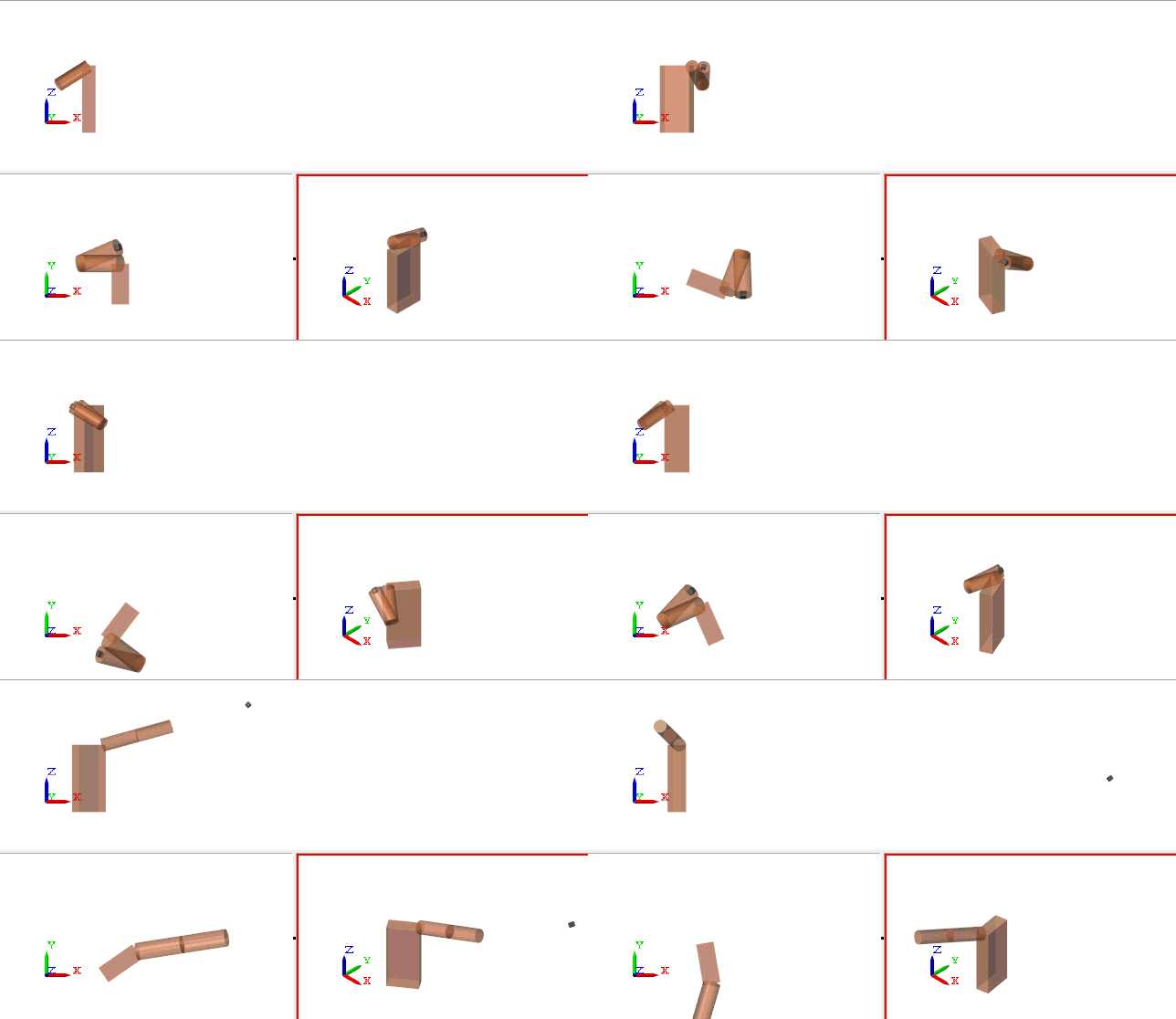
Top level of the shot put simulation

This model focuses on the spin and the push. To model the spin phase, we attached a Body block to a Revolute Joint. This is similar to the Olympic figure skater model from the last winter Olympics.

Using a series of Rigid Transforms and Revolute Joints, we implemented the shoulder, upper arm, elbow and lower arm. I decided to actuate the elbow and shoulder by motion. That way, we can focus on the kinematics of the throw, and measure the forces required to generate the motion to ensure they are realistic.

The tricky part is in the subsystem called "Lockable 6-dof Joint". During the spin and the put, the shot must move with the hand. Once this is complete, the shot must "fly" by itself until it hits the ground.

Simscape Multibody has a set of Constraints blocks, but those cannot be enabled and disabled during simulation as we need here. To implement the release of the shot, we use something similar to a stiff spring and damper, that we turn off when the shot gets released. For that, we sense the position and velocity of all the degrees of freedom of the 6dof Joint, multiply by stiffness and damping coefficients, and apply the results as forces and torques.

Locking a joint in SimMechanics

Control

Now that we have a moving arm and and spinning body, we need to figure out how to make it move.

Before going for an optimal move, I thought it would be convenient to use Stateflow to make a first quick test. Using a series of 4 states, we can make our thrower going through the phases of spinning, pushing with the shoulder, pushing with both elbow and shoulder, and releasing the ball.

Arm motion logic

As you can see below, it works! With a 10.12 meters shot, we are far from a gold medal, but it's a good start.

Animated shot

Now it's your turn

Anybody interested in designing the perfect throw?

Download the model, and give it a shot. I am sure this could make a very interesting optimization problem. I would start with fmincon to try maximizing the distance while respecting constraints like maximum torques at shoulder and elbow, and landing in the valid area. At the end, we should be able to reproduce a world record shot that looks like that:

the Dream Shot

Have fun, and enjoy the Olympics!

Olympic 2016 – Pole Vault

$
0
0

For this second post in our Olympics series, I am happy to welcome guest blogger Amit Raj to describe how he simulated the pole vault competition.

Introduction

Track and field events are one of the most popular kinds of athletic sports in the Olympics. Pole vaulting is a track and field event where an athlete uses a long flexible pole as an aid to jump over a bar. Historically pole vaults were used to jump over canals and marshes. Pole vaulting has featured as an event in the Olympics since 1896.

Pole Vault

Image source: https://polevaultphysics.wikispaces.com/The+Physics+of+Pole+Vaulting

Conservation of Energy

Vaulting is a prime example to demonstrate the conservation of energy principle. The athlete builds up kinetic energy and uses the pole to convert this into potential energy.

Concervation of energy

The current world record stands at 6.14 m set by Sergey Bubka. The record for fastest sprint is by Usain Bolt, at a little over 12 m/s. However, vaulters need to sprint with the weight of the pole. If we are reasonable and assume a sprint of 10m/s, that gives us a height of:

Height equation

This is the change in height of center of mass. If we assume an initial height of center of mass at 1m we have a height of 6.102 which is pretty close to the world record.

Physics works... Yeah!

The phases

Although speed is important to determine the height, the technique of the vaulter also decides how effectively all the kinetic energy can be converted into potential energy. The conversion usually happens in multiple stages.

The generally accepted model for pole vaulting consist of the following phases:

  • Approach: During this phase the athlete tries to maximize his speed along the runway to achieve maximum kinetic energy
  • Plant and take off: The athlete positions the pole into the “box” to convert the kinetic energy into stored potential energy in the pole
  • Swing up: The athlete moves the swing leg forward and tries to keep the pole bent longer to achieve an optimal position for the
    release
  • Turn: The vaulter spins 180 towards the pole while extending the arm
  • Fly away: The vaulter releases the pole and falls back on the mat under the influence of gravity

Let's now see how we can simulate that.

The Model

We model the above phases using three main stages – The run up, take off and release. In Simulink, each stage is a If Action Subsystem governed by its own set of dynamic equations. The challenge lies in switching between the different dynamics and still maintaining continuity.

Pole Vault model

The first phase is quite simple, we just run at a constant speed of 10 m/s. The important thing to note here is the usage of the state port.

The Run

When the If condition changes from the running subsystem to the takeoff, the state ports of the Integrator blocks write to Goto blocks. In the Takeoff subsystem, we can then use From blocks to receive the final state of the run to initialize the takeoff subsystem.

In this case, the run was computed in a Cartesian coordinate system, but we decided to implement the takeoff in a polar coordinate system. Solving the equation for the bending of the pole is simpler in polar coordinates, where the integrated states are the length and angle of the pole.
Takeoff

Once the pole reaches 90 degrees, it is time to let it go and switch to the flying phase.

In a similar manner as the previous transition, we pass the final states through Goto and From blocks. In the flight subsystem, we convert back to Cartesian coordinates and let the gravity do the work.

Flying

Here is what the final trajectory looks like:

The Trajectory

Now it's your turn

Download the model here, and try different parameters to see what is the optimal configuration to win the pole vault competition at the Olympics.


Including a mask image in your block

$
0
0

Earlier today, a colleague came to me asking for a way to include an image in a block to be used as mask image. I though it might be interesting to share my response here.
The Problem

Here is the question I received:

I want to mask a block and display an image on the mask. The image is stored in a .PNG file. When I will distribute the block, I would prefer sharing only a Simulink file, and not the image.

The Solution

As described here, it is possible to use the image function to read and display an image file on a block mask. However, with this technique the image must be on the MATLAB path.

To avoid the need to carry the image file, it is possible to associate the image data with the block.

Associating image data with blocks

It is important to explicitly make the UserData persistent, otherwise it will not be saved with the model. I also like to make the UserData a structure. That way if someone else wants to save data there, it will be possible to create a new field.

Once this is done, the image data will stay with the block. You can copy it to a different subsystem or to a new model, it will remain associated with the block.

Once the data is associated with the block, you can retrieve it in the mask icon drawing commands, and display it:

Displaying the Image

Now it's your turn

How are you displaying images in your masked subsystems? Let us know by leaving a comment below.

What’s new in R2016b!

$
0
0

MATLAB R2016b is available for download since yesterday, so today I decided to highlight the most visible enhancements in the Simulink area.

Property Inspector

From the View menu or using the shortcut Ctrl+Shift+I, you can launch the Property Inspector.

When selecting a block, the parameters that you normally view and set in mask dialogs are displayed and can be modified. This should make it easier and faster for you to see and modify block parameters.

Property Inspector

Note that the Property Inspector is by default on the right of the canvas, but can be dragged at the bottom, right, or top if you prefer.

Model Data Editor

With the same goal of making it easier to access and configure models, we also added the Model Data Editor.

In a table, it gives have access to all the parameters, signal and data stores in a subsystem. For example, in the Signals tab, you can enable/disable logging, or set the code generation properties of all your signals.

Model Data Editor

Just-in-Time Acceleration builds

Before R2016b, we used to generate C code and create a MEX-file for model running in accelerator mode. As we did for Stateflow in R0215a, Simulink now uses a Just-in-Time (JIT) compilation technology to improve initialization time of models running in accelerator mode.

It will probably go so fast that you will not be able to see it, but you might notice the following status in your model while Simulink is "jitting" your model:

Accelerator Just-in-Time compilation

Updated fonts and block icons

Here is a comparison using a few blocks between R2016a and R2016b.

Improved Fonts and Icons

Edit-Time Checks

If we can detect it, why wait for you to click the play button to tell you that there is a problem?

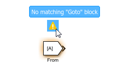
In R2016b, you might notice new colors and exclamation marks on GoTo, From and Data Store Memory blocks if we detect mismatch or duplicates.

Now it's your turn

Give a look at the R2016b release notes and let us know which new feature or enhancement you prefer or would like to read about on this blog.

Simulink Student Challenge 2016

$
0
0

Today we are having a quick post to highlight the 2016 edition of the Simulink Student Challenge

Simulink Student Challenge

You are a student and you are working on a project involving Simulink? Create a video describing your project and how you are using Simulink, and post it on youtube with the tag #SimulinkChallenge2016. You could win up to 1000$.

Past Editions Entries

Let's look at a few videos from past editions:

Vehicle Dynamic Controls for an electric race car

The MAMMOTH Rover

Simulating Human-Piloted Helicopters with Suspended Loads

Automatic flight in GPS denied areas

Control system to track and regulate the travel, pitch and elevation angle of the helicopter

Now it's your turn

Submit your entry to the 2016 Simulink Student Challenge before December 18th 2016 for a chance to win!

New in R2016b: The Finder

$
0
0

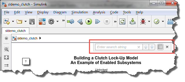
The first time you will try searching for blocks or parameters in MATLAB R2016b, you will notice that the interface of the Find Tool has been completly re-designed.

Try hitting Ctrl+F in a model, here is what you will see:

Finder

Type something in the search box and hit Enter, all the results in the current subsystem will be highlighted. The first item found will be highlighted bolder than the others, and clicking on the Up and Down arrows will navigate between all the objects found.

Highlighted Found Blocks

If you want to see a table listing all the items found, click the View In Finder button

View In Finder

A table, docked in the editor, will appear. You can drag the table, up, down, left or right of the canvas, or undock it if you prefer. Here is what it looks like at the top:

Finder docked in model

Advanced Maneuvers

If you need to refine the search criteria, click the advanced search button:

Advanced Search

With the Advanced Search Setting dialog, you can control what to search and where to search for.

Advanced Search Settings

A few tips

Before giving tips, I need to warn you of little something...

Warning: In R2016b, there is a typo in the Advanced Search Settings dialog. The search criteria "Search block diagram parameters" should say "Search block Dialog parameters".

Tip 1: If you have a large model and you are searching for blocks or signals, disable the Search block Dialog parameters option. this will make the search significantly faster.

Tip 2: Left of the search field, there is a button to decide if you want to search in the current system only, or everything below. As you can imagine, selecting the appropriate scope will help performance.

Tip 3: When searching for property values, there is an "Other" field, where you can type any block specific parameter. For example if I want to find all the Integrator blocks with External Reset, that would look like:

Advanced Search Settings Parameter value

Now It's your turn

I hope the new finder will help you finding what you are looking for more efficiently. Give it a try and let us know what you think.

Creating iPhone and iPad Apps with Simulink

$
0
0

The other day, a user told me: That would be cool if we could program apps for smartphones using Simulink.

Guess what my answer was: Of course you can!

Simulink Support Packages for Apple iOS and Android

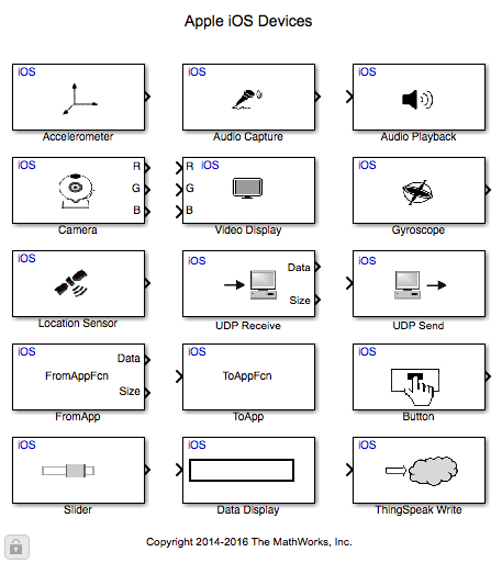
Yes, you heard it right. If you have a Simulink license, you can download the Simulink Support Package for Apple iOS, or if your prefer the Simulink® Support Package for Android™.

Simulink Apple iOS library

Since he works mostly in the Apple ecosystem and I don't, I asked my colleague Mariano Lizarraga Fernandez to be guest blogger this week and describes his first experience trying to build an app for his iPhone.

Getting Started

Before you get started, make sure you have the following:

  • An Apple computer running OS X Yosemite or El Capitan with MATLAB and Simulink installed.
  • Xcode 7.x.
  • A free Apple Developer Account.
  • The Simulink Support Package for Apple iOS.
  • An iOS device running iOS 8.x or 9.x.

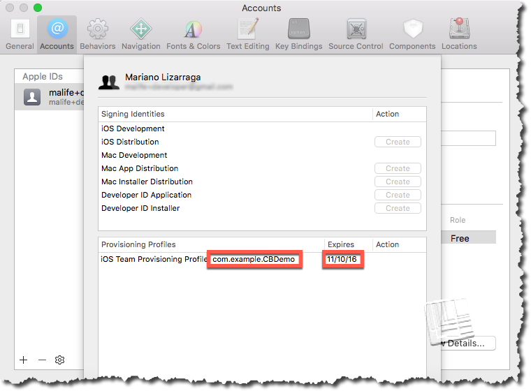
Make sure that when you install the Support Package you completely follow the setup instructions including obtaining a certificate for signing the application. You need to make sure, in your Xcode preferences, that your certificate is valid and that the identifier matches that of your application. In the following picture, CBDemo is the name of the Simulink model:

Xcode Configuration

For your first model, as suggested in the Getting Started documentation page, an easy test is to acquire the camera video, and display it on the screen. You can directly access this demo by executing iosGettingStartedExample in MATLAB.

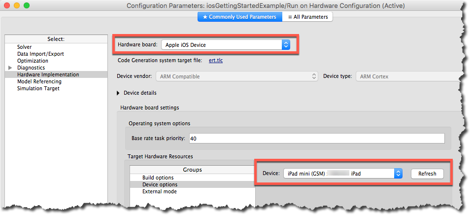
Before running this model, open the model's Configuration Parameters, and in the Hardware Implementation section make sure the Hardware Board is configured for Apple iOS Devices and that your iOS Device is shown in the Target Hardware Resources:

Model Configuration for iPad target

Now to the Fun Part ...

To give you an idea of what kind of app it is possible to create, we decided to start with an example from the Computer Vision system Toolbox: Traffic Warning Sign Recognition

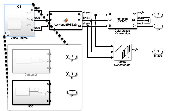
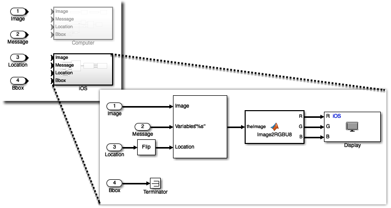
The model as-shipped loads a video from your filesystem and performs identification of stop and yield traffic signs. To adapt it for the iOS target, we only need to replace source and sink. Instead of just replacing the blocks, we decided to use Variants Subsystems to switch between a simulation-only version, and a deployable version.

For the source, we use the iOS camera source block. Since this source only produces 8-bit unsigned integers, we need to modify: (1) How the From Multimedia File block produces the output so it too results in 8-bit unsigned integers; and (2) Convert the 8-bit frame to single precsision floating point one using the im2single function.

Video source for Simulink Apple iOS library

Similarly, for the sink variant, since the iOS Video Display block only accepts 8-bit unsigned integers, we convert the processed image from single precision floating point to 8-bit unsigned integers using the im2uint8 function

Video Sink for Simulink Apple iOS library

Here is what this looks like in action on an iPad mini:


https://youtu.be/AMLdghppCn4

Now it's your turn

What kind of app will you create for your iPhone or iPad? Noise cancelling headphone? Driving assistant for blind people?

If you create a cool app, submit it to MATLAB Central File Exchange and let us know in a comment below.

Export Function Models

$
0
0

I started writing this post with the goal of talking about the new Initialize Function, Reset Function and Terminate Function blocks, along with the closely related State Reader and State Writer blocks introduced in R2016b.

However I quickly realized that those new features are very closely related to a type of model architecture I almost never talked about on this blog: Export Function Models.

Generating Code

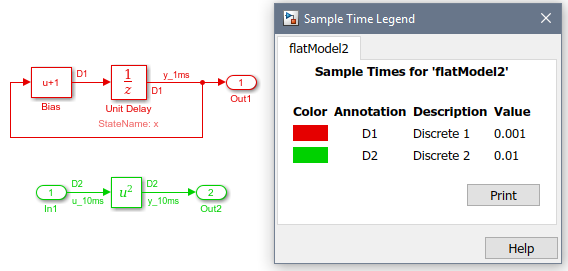
Let's use the following model as example. It contains a Bias and Unit Delay block executing at 0.001s and a Math Function block executing at 0.01s.

Simple Example model

As you all probably know, with Embedded Coder it is possible to generate C code from a Simulink model. Using the default Embedded Coder System Target File, the code you will get will look something like:

Code Generated from Simple Example model

As you can see, the code is made of one Initialize function, and a Step function. The step function is designed to be called at the model base rate, 0.001s in our case. Perfect to execute the code in a single-tasking context.

If you prefer, you can ask Simulink to Treat each discrete rate as a separate task.

Multi-Tasking

In this case, the generated code will be composed of one function par sample time. It is then possible for you to implement the scheduler and call each rate the way you want.

Multi-Tasking Code

Exporting Functions

Having one function per rate is useful, but what if you want more control over the execution of the code? For example, you could want one rate to be divided into multiple tasks, and assign different priority to each of them.

For that, Embedded Coder offers the possibility to export functions. Exporting functions provides direct control over the generated functions and the ability to simulate their scheduling and prioritization.

To be compatible with the concept of export functions, your model must be built in a specific way: The top level of the system for which you want to export functions must contain only Function Call Subsystems, Inports and Outports. That way, one function per subsystem will be generated.

For our example model, we can rearrange it that way:

Export Function Subsystem

For simulation, the scheduling of the different tasks must be done explicitly, for example using Stateflow as in the above image. When time comes to generate code, you can right-click on the subsystem and export the functions:

Export Function Subsystem Model

The code will look like the following:

Export Function Subsystem Code

And you will be able to include this code in your hand-written scheduler. As mentioned above, this would allow you to divide one rate into multiple functions, or tasks.

Export Function Model

For large projects, it is also possible to create Export Function Models.

In this case, the top model will be used for simulation only, and you will generate code for the child model. Simulink will automatically recognize that the model is designed to export function, and the code will be similar to the one generated from the subsystem above.

Export Function Model

What's next?

Next week, we will see how the new Initialize Function, Reset Function and Terminate Function blocks can be used inside export function models to simulate the shutdown and restarting of the function or task.

State Reader and State Writer blocks

$
0
0

As mentioned in my previous post, I have been trying for some time to write about the new Initialize Function, Reset Function and Terminate Function introduced in R2016b. However, every time I end up realizing that I need to introduce another feature first.

This week: The State Reader and State Writer blocks, also introduced in R2016b.

Not your everyday standard block...

Let's begin with a simple model where I have a Discrete State-Space block.

Discrete State-Space

I can add to the model a State Reader block, open its dialog, and select the Discrete State-Space block to read its states. Notice the diamond shaped "x" on top of the Discrete State-Space block. It is there to indicate that its states are being read somewhere else. Also, notice the block name next to the State Reader, indicating where it is reading from.

Selecting block to be read by the State REader block

You probably also want to notice that the State Reader block is highlighted in red. This is thanks to a new feature in R2016b: Edit-Time Checking. If you hover the mouse on top of the block, you will get more details:

Edit Time Check

Hmm... What does that mean? What's wrong with putting those two blocks in the same subsystem?

As I said, the State Reader and State Writer blocks are not like every other block! Let's try to update the diagram. This time we receive this error:

State Reader Error

The Explanation

For those of you reading this blog for a long time, I hope you remember a post I wrote many years ago titled How Do I Change a Block Parameter Based on the Output of Another Block?

In this post, I explained that if a block could change the parameter of another block, this would lead to unpredictable sorted order. During one time step, no one could predict if the parameter would be modified before or after the block executes.

A similar reasoning applies to the State Reader and Writer blocks. Since there is no signal connecting the Reader/Writer to the state owner, there is no explicit data dependency to enforce the sorted order. This is why those blocks can only be used in contexts where the execution order is explicitly specified by the user.

In other words, this "constraint" is a good thing, designed to make your life easier on the long run.

Let's look at those constructs where the State Reader and State Writer blocks can be used.

Mutually Exclusive Subsystems

In a manner similar to how the Clutch Lock-Up Example uses the State port of the Integrator block, it is possible to use the State Reader and State Writer block to pass states between conditionally executed subsystems.

A simple way to illustrate that is to implement the equation of two falling masses rigidly linked together; that suddenly separate. In the first part of the simulation, the motion is computed using two Discrete-Time Integrator blocks in series.

Combined Masses

In the second part of the simulation, we use two series of Discrete-Time Integrator blocks, initialized using the State Reader block, configured to read the state of the Integrator blocks from the first part of the simulation

Split Masses

At the top level, the simulation looks like:

Top Model

Export Function Models

Using an Export Function Model like the one described in my previous post, you can explicitly control which block executes first.

Begin by creating a model with two Function-Call Subsystems, one for the Discrete State-Space, and one for the State Reader:

Export Function Model

You can then use this model as a referenced model, where the parent explicitly schedules the order into which the Discrete State-Space and the State Reader blocks are executed

Export Function Top Model

Branched Function Call

This syntax is similar to the previous example, except that everything is in the same model.

Function Call Scheduler

What's next?

It is important to realize that the examples above using the branched function call and the Export Function Model are too simple to really illustrate the real power of the State Reader and State Writer blocks. They are the simplest models I can think of to illustrate the usage of those blocks.

In a soon to come post, I will show how to combine these features with the Initialize Function, Reset Function and Terminate Function in a more realistic use-case.


Using Simulink Functions to Simulate Hardware Services

$
0
0

This week, I want to introduce another feature that becomes useful when combined with the Initialize Function, Reset Function and Terminate Function blocks.

In R2014b, Simulink Functions got introduced. In this post, we highlighted how Simulink Functions can be used to create an Export-Function model. In this case, the Simulink Functions are placed inside a model. In simulation, you can reference the model and call the functions using the Function Caller block.

Simulink functions used as function library

You can then generate code for the function library model and call those functions in any way you want from hand-written code.

The opposite

One thing we did not mention at that time, is that it is possible to use Simulink Functions and the Function Caller block in completely opposite way, where the referenced model has a Function Caller block, calling Simulink Functions present in the top model.

Simulation harness

Why would someone want to do that? In short, the answer is to simulate custom code that is not directly available for simulation. Let's see how this works.

Using the Function Caller block to call external code

If we generate code for the child codeGenModel.slx in the above picture model, the code will look like:

Generated Code

By default, this code would not build, since the compiler would not know where to find the function timesTwo. However, if you configure your model properly, the function timesTwo can come from anywhere you want. For example, it could be in a dynamic library against which you will link to on your embedded target. For this example, imagine that there is a timesTwo service available in this timesTwo.c file:

Custom Code

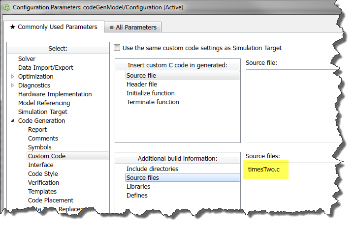
In the model configuration, I specify that this file should be included in the build process:

Custom Code Configuration

This allows me to generate an executable that calls my custom timesTwo.c implementation.

Conclusion

To summarize, the idea is to create a Simulink Function that emulates the behavior of external software. You can build a simulation harness model that references your code generation model and it will see the Simulink Function. When time comes to generate code for the child model, it will have no idea the Simulink Function exists, but instead will link against any external code you specify.

It is important to note that this technique is just one way to include custom code in the code generated from Simulink.

If the custom code was available on the host, I would recommend going with an S-Function to wrap and reuse the same custom code both in simulation and code generation.

However if the code is unavailable, for example because it is available as an OS service on the target embedded processor, this approach can be interesting.

What's next?

Now that we have introduced the concepts of Export Function models, the State Reader and Writer blocks, and this way of using Simulink Functions, I believe we have all the pieces to make a realistic example illustrating how we see the Initialize Function, Reset Function and Terminate Function blocks being used... next week.

Simulating the Startup and Shutdown of your software

$
0
0

This week, we are finally diving into the Initialize Function, Reset Function and Terminate Function blocks.

As a starting point, I recommend looking at this video about Initialize and Terminate Functions by my colleague Teresa Hubscher-Younger.

Simulating the Startup and Shutdown of the Generated Code

In this previous post about Export Function models, we have seen how we can simulate a model configured to export functions: by referencing it using a Model block.

In this example, we were able to simulate the behavior of the code being run once. In other words, if the code will be running on an embedded controller unit (ECU), what this model simulates is that the ECU boots up when the simulation starts, the code runs, and the ECU shuts down when the simulation terminates.

This is interesting, but what if you want to simulate a larger scenario, where the ECU is booted up and shut down multiple times? This is what the Initialize Function and Terminate Function are designed for.

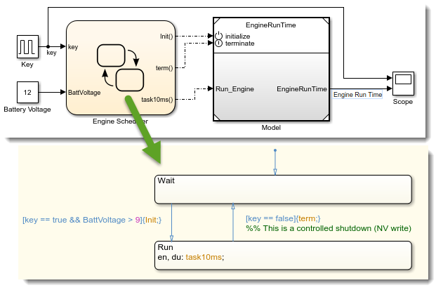
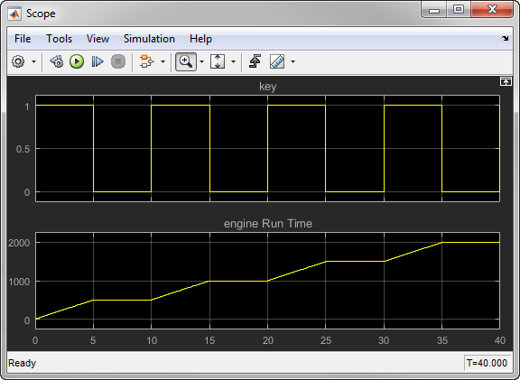
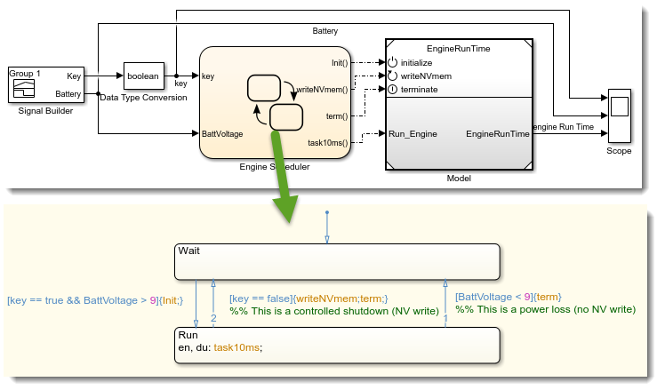
What Teresa's example does is simulating a car being started and shut down multiple times, due to two different conditions. When the car is running, we are incrementing a counter to keep track of how long the engine has been running, in its entire life. In a normal shutdown case, when the key is turned off, we need to write the total run time in a non-volatile memory, so it can be retrieved next time the car is started. In case the battery dies, the car also shuts down, however in that case we don't have time to write to the non-volatile memory.

Let's see how to make that happen!

Enabling Initialize and Terminate Events

Let's begin with a simple export-function model implementing a counter.

Export Function Counter model

In R2016b, you will notice that when you reference a model setup to export functions, the dialog of the Model block includes two new options.

Model Reference Dialog

When you enable those, the model block will show two new ports, to which you can connect function-call signals. As a first simple test, let's make a Stateflow chart to start and shut down our counter when the key is turned on or off:

Model Reference with init and terminate ports

If we look at the results, we can see that the counter increments when the key is on, and stops when it is off. When the key passes from off to on, the counter gets reset.

Model Reference with init and terminate ports

Custom Initialization and Terminate Events

As described earlier, we do not want the counter to reset at every shutdown. To keep the counter value, we can use Intialize Function and Terminate Function blocks. Inside the Terminate Function, we use the State Reader block to obtain the current counter value and store it into a Data Store block. Similarly, inside the Initialize Function, we will read the Data Store block and use it to initialize the counter.

Model Reference with init and terminate ports

Now when we look at the results, the counter keeps increasing after being shut down and restarted.

Model Reference with init and terminate ports

Reset Function

As mentioned previously, we also need to handle the case where the vehicle shuts down because of low battery voltage. This means that we do not want to write to the Data Store every time the model terminates.

To do that, we can change Event Type in the Terminate Event Listener block from Terminate to Reset and give it a meaningful name. In that case, since the model does not have a Terminate Function block anymore, the default blocks terminate function will be executed when the simulation harness will trigger the terminate event.

Reset Function

We update the Stateflow Scheduler to cover both shutdown cases:

Model Reference with init and terminate ports

Note that in the above model, in the Model reference parameter dialog, we enabled the "Show model reset port(s) option". This is what gives us the additional writeNVmem port.

When looking at the results, we can now see that if the shutdown is caused by a battery failure, the counter value is not kept for the next restart.

Model Reference with init and terminate ports

Code Generation

Now that we have a simulation that behaves as expected, let's look at configuring code generation.

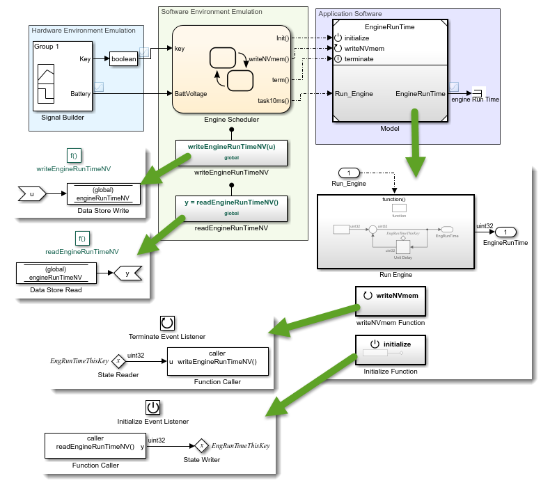
In the generated code, writing to the non-volatile memory very likely needs to be done using custom code or hardware services provided by the embedded target. To deal with that, we will use Function Caller blocks and Simulink Functions in the way highlighted in this previous post.

To resume in a few words, we replace the Data Store blocks by Function Caller blocks in the export-function model. To get the simulation behavior, we use Simulink Functions implementing the same logic as previously done in the Initialize and Terminate Functions, reading and writing to data store blocks.

Here is what the overal contraption looks like:

Code Generated from Export Function Model

As described in this previous post, for code generation, it is possible to specify in the configuration of the export-functions model where the functions writeEngineRunTimeNV and readEngineRunTimeNV should be found at linking time.

If we generate code for the Export Function model, what we get looks like:

Code Generated from Export Function Model

Now it's your turn

Let us know what you think of this semantics by leaving a comment below.

What’s New in R2017a!

$
0
0

MATLAB R2017a is now available for download. For this first post about R2017a, I want to highlight features that will help you creating models more efficiently.

Simplified Subsystem Bus Interfaces

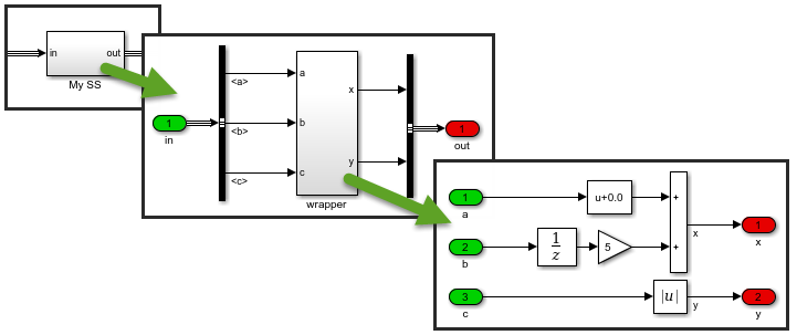
I often receive large models from users where subsystems and buses are arranged like the following. By using a wrapper virtual subsystem, this pattern helps to avoid line cluttering.

Bus before

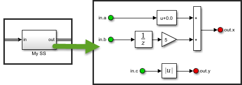
In R2017a, thanks to the new bus element ports, your Subsystems can now look like this:

Bus R2017a

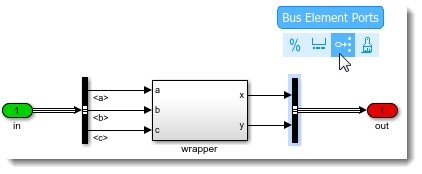
If you want to convert your existing models to this new semantics, we also added a functionality to do the conversion automatically:

Bus Conversion

Improved Parameterization of Referenced Models

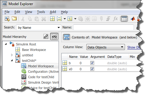
For those of you who need to pass arguments to referenced models, you will notice the new Argument column in the Model Explorer when creating new variables in the model workspace:

Model arguments

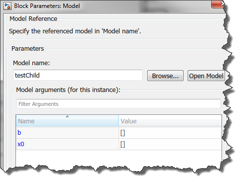
When referencing the model, the dialog of the Model block will list the variables marked as Arguments and allow you to specify their value. For those of you with many arguments, notice that the table is searchable and sortable.

Model arguments values

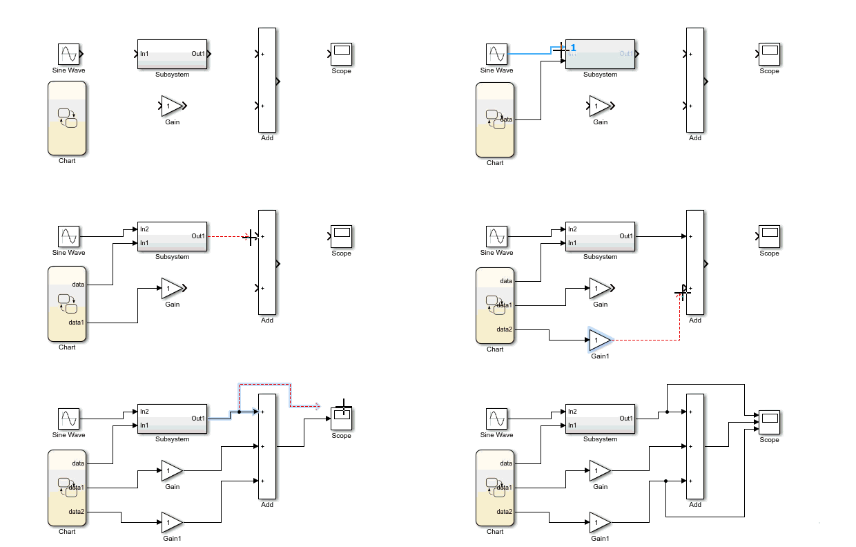
Automatic Port Creation

In R2017a, you can simply drag a signal line close to a block and a new port will automatically appear. The best way to describe this feature is to see it in action:

Automatic Port Creation

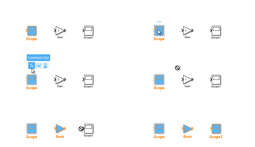
Format Painter

Easily apply the formatting of one block to other blocks using the format painter:

Format Painter

Now it's your turn

Those are some of the features added in R2017a to help you editing model more efficiently. There are many other exciting new features I will be blogging about soon.

Look at the release notes, and let us know in the comments below what is your favorite new feature, or which one you would like to read about on this blog.

Simulating models in parallel made easy with parsim

$
0
0

Some time ago, I wrote a series of posts to highlight the different factors to take into account when trying to run simulations in parallel. In R2017a, we are making it significantly easier with the introduction of a new function: parsim

Let's see how that works!

Simulink.SimulationInput

If you are going to use the Parallel Computing Toolbox to simulate a model multiple times, there is obviously something you want to change to make each run different. This is done through the Simulink.SimulationInput object.

By creating one Simulink.SimulationInput per simulation, you can define the properties specific to each run, including initial states, model parameters, block parameters, input signals, and variables used by the model.

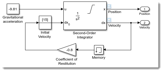
Let's take this simple bouncing ball model, and try to simulate it in parallel for different coefficient of restitution.

Bouncing ball

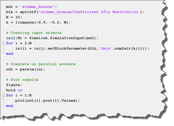
In this case, we will simulate the model for 10 different values, from 0.2 to 0.9. For that, I create an array of 10 Simulink.SimulationInput objects, and use the setBlockParameter method to specify the coefficient of restitution for each simulation. I can then simply pass this array of Simulink.SimulationInput to parsim, and I will receive as output an array of Simulink.SimulationOutput objects.

Parsim simple example

A More Realistic Example

Let's make this bouncing ball example more realistic by adding the following:

Workspace Variables: Before parsim, one of the challenges when simulating a model in parallel was to manage the variables needed by the model. I tried to provide tips and tricks to help with that in this previous post. For our bouncing ball example, instead of hard-coding the value of parameters like gravity and coefficient of restitution in block dialogs, let's have those be variables in the MATLAB base workspace, created by a MATLAB script.

Bouncing ball Model with workspace variables

Output Processing: In most cases, a simulation produces a large amount of data. If you are simulating on a remote cluster, you probably want to avoid transferring all this data. Instead, you can post-process the logged data and reduce it to what you are really interested in.

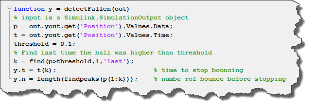
For the post processing, we need to create a function that receives as input the simulation output object and returns a structure output. For example, I can use the logged position to computer how long it took for the ball to stop bouncing, and how many rebounds it did.

Post Simulation Function

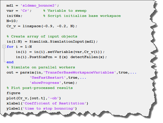
With that setup, we can create our array of Simulink.SimulationInput object, and use the setVariable method to specify different values for the workspace variable Cr. For the post-processing function, we specify a handle to it to the postSimFcn property of the simulation input object.

Here is what it looks like:

Parsim example

Notice how I also use the UseFastRestart option to speed things up even more by compiling the model only once on each worker.

Handling Errors

One of the thing I like about parsim is how it behaves when the simulation errors out.

In this case, the Simulink.SimulationOutput object contains all the logged data until the error happened, and a ErrorMessage field describing the cause of the error.

Parsim error output

This is very useful to understand what went wrong without the need to re-simulate the model.

If you cannot figure out what went wrong based on the logged data, you will very likely want to add more instrumentation to the model and re-simulate it on your host machine. In that case, you will like the applyToModel method of the simulation input object. As its name implies,
this method will configure your current MATLAB session and model so that you can simulate it as it did on the worker.

Now it's your turn

Give a try at the new parsim function in R2017a and let us know what you think in the comments below.

Improved Behavior of Auto Tolerance in R2017a

$
0
0

Are you familiar with the meaning of auto for the Absolute tolerance of Simulink variable-step solvers?

In R2017a, we decided to change the meaning of auto for the Absolute Tolerance... If your model is using this setting, I recommend you keep reading to see if and how you might be affected.

Absolute Tolerance

How Tolerances work?

To learn more about how error tolerancing works for Simulink variable-step solvers, I recommend going through this documentation page.

What you will find is that for each continuous state in a model, an error is computed. This error is computed differently for each solver, but in general variable-steps solver integrate continuous states using two methods, and the error is the difference between both.

If we take the simplest of our variable-step solvers, ode23, it computes its output y(n+1) using a third-order approximation and also computes a second-order approximation z(n+1) so the difference can be used for error control and adapting the step size.

ode23

To see that in action, I recommend using the Simulink command-line debugger, in particular a combination of strace 4, trace gcb, and step top.

Once the error is computed for each state, we ensure that the error is smaller than the absolute tolerance, or the relative tolerance multiplied by the state amplitude, whichever one is the largest.

Error Control

Over time, this can look like this:

Error Tolerances

What's new in R2017a?

Before R2017a, when choosing a value of auto for the absolute tolerance, the initial value used was systematically 1e-6. Then if the amplitude of the states increases during the simulation, the absolute tolerance would also increase to a value corresponding to the state value multiplied by the relative tolerance.

In R2017a, the meaning of auto for absolute tolerance is changed to the value of the relative tolerance multiplied by 0.001. We believe that this new definition of auto reduces the chances of getting inaccurate results.

To illustrate the difference, let's take this simple model implementing a first order transfer function:

First order step response

In R2016b, if I set the relative tolerance to 1e-6 and leave the absolute tolerance to auto, the results look like:

First order step response

As you can see, this result is far from accurate, a first order transfer function should not overshoot like that. The problem is that the value of the state is smaller than 1e-6, and the absolute tolerance decided by "auto" is 1e-6. With such setting, pretty much any answer would be within tolerances and considered valid.

In R2017a, when I simulate this model the results I get is:

First order step response R2017a

With the new definition of "auto", the absolute tolerance used is now relTol*0.001 = 1e-9, giving the expected answer.

Consequences?

In R2016b and prior releases, you might have ended up setting the relative tolerance to a value much smaller than 1e-3, while leaving the absolute tolerance to auto. This would have compensated for the lack of accuracy due to the auto absolute tolerance being always larger than 1e-6.

In R2017a, the lower bound on auto absolute tolerance is no longer fixed at 1e-6. In case this tighter tolerance slows down your simulation, the first thing I would recommend is leaving the absolute tolerance to auto, and try increasing the relative tolerance close to its default value of 1e-3 (or 1e-4) to get results of comparable accuracy.

You may also want to try different values for relative and absolute tolerances and see what gives the best trade-off between performance and accuracy for your model.

Now it's your turn

Let us know in the comments below if you are impacted by this change, we would like to hear.

Viewing all 159 articles
Browse latest View live