I am not done yet... there are still a few more new things in Simulink R2015b I need to highlight.

Scope

In R2015b, the Simulink Scope has been entirely redesigned with tons of new features. It looks a lot closer to the Time Scope from the DSP System Toolbox.

Visualization of Auto-Inserted Rate Transition Blocks

If you are familiar with the option Automatically handle rate transition for data transfer, you will like the addition of new indicators showing you where those are inserted and what operation they are doing. If you hover over the indicator, it will offer to insert the block for you.

Dataset logging format is everywhere!

To help standardize your post processing scripts, most methods of logging data from a model now default to use the Dataset format

Referenced Simulink Projects

Since the first day Simulink Projects was released, we have been asked if a large project could include or reference smaller Simulink Projects. It is now possible. From the Simulink Project tab, click the References button to add or remove referenced projects.

From the Project Shortcuts tab, you can run the shortcuts of your referenced projects.

Visit the Componentization of Large Projects documentation page to learn more about this topic.

Configuration Parameters List View

Next time you open the Configuration Parameters of a model, notice the two buttons at the top. Category is the view you have been used to seeing over the years. List gives you a completely new way to find and tune the parameters you need.

Now it's your turn

Let us know what you think of those new features by leaving a comment here.

Do you run the Upgrade Advisor on your models when upgrading to a new release? If not, you should!

Upgrading a model to a new version

Today, I want to show how the Upgrade Advisor can help when transitioning to a new version to take advantage of new features, as well as the reasons behind some of the changes we’ve made that require upgrading.

To show this, I launched MATLAB R2007b and made a Simulink model with a few blocks.

I open it in the latest release, R2015b. I am able to simulate it without errors, but I will use Upgrade Advisor to see if new changes introduced since R2007b affect this model.

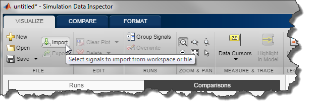
The Upgrade Advisor is launched from the Analysis menu:

You will notice that it looks very much like the Model Advisor... because it is based on the same technology. It contains different checks, targeted at helping you to upgrade to new versions.

I enable all the checks and run them all. Here are the results:

Wow... 8 warnings! Let's see what those are.

Check usage of function-call connections

In the past, the default value of this diagnostic setting was "Use local setting". Since then, we realized that allowing that was sometimes leading to non-deterministic model execution. Now we recommend to always set this diagnostic to "Error".

This can easily be fixed by clicking the "Modify Settings" button below the check result

Check that the model is saved in SLX format

In R2012b, we introduced a new Simulink file format with .slx extension. This format provides a lot of advantages compared to the old .mdl format. The files generated are usually 10 times smaller, better support for non-English characters like Chinese and Korean, and some recent features are supported only in this mode.

Once again, this can be fixed by a single button click.

Check signal logging save format

In R2007b, signals were saved in ModelDataLogs format. Since then, many bugs and usability issues have been found with this format. We decided to address this issue by creating a completely new logging format, the Dataset.

You can see an example problem with the old ModelDataLogs format in Bug Report 495436.

If you are ready to move to the Dataset format, the action button will do it for you.

Check model for block upgrade issues requiring compile time information

This one is very important. Since R2007b, we decided to deprecate the 1D Lookup Table block and to replace it with the n-D Lookup, configured with one dimension.

If we compare the dialog of the two blocks, we can see that the new one offers a lot more options, like spline interpolation. The new block also has improved performance, both in simulation and generated code.

Many other blocks can be found by this check.

Merge, Buses and Simplified Initialization

The next 3 checks are closely related. As was the case for Check usage of function-call connections, we realized since R2007b that some semantics in Simulink can lead to results that are difficult to understand.

To help with that, we decided to discourage, and in certain case completely disallow, certain practices like mixing buses and muxes, allowing multiple writes to the Merge block during the same time step, etc.

If you are lucky, your model did not contain such patterns and you will be able to apply the recommended settings easily. If your model contains such pattern, the results of those checks will guide you on how to manually modify the model if it cannot be done automatically.

Analyze model hierarchy and continue upgrade sequence

If the model contains library blocks or referenced models, this last check will re-run the Upgrade Advisor on those, until the entire hierarchy is updated.

Note that in R2015b, a bug got introduced in this last check. I recommend installing the patch attached to Bug Report 1307296 to avoid it.

Now I have a clean model fully updated

Now it's your turn

I hope you learned a few things about why it is important to run the model through the Upgrade Advisor when moving to a new release. Without the Upgrade Advisor, there are multiple things that I could have missed, and might have caused me trouble later.

Let us know what you think of the Upgrade Advisor by leaving a comment here.

About a year ago, I read the book The Martian, by Andy Weir. I really enjoyed the story, with all the technical details of how Mark Watney solves one problem after another to survive alone on Mars.

A few weeks ago, I realized that a movie with Matt Damon was coming out. After watching a few trailers, I ran into this YouTube video where Adam Savage (from the TV show MythBusters, among other things) interviews Weir.

In this video, Weir describes how he did not explicitly give the launch date of the Ares 3 mission in the book, but left enough clues for someone to figure it out.

As you can imagine, the nerd in me could not restrain itself from taking on that challenge. In this post, I will describe how one can use MATLAB to figure out the launch date of the Ares 3 mission.

Finding the launch date

In the book, we can find the following reference points:

1. Thanksgiving: One of the main plot elements is that Mark Watney is able to extend his stay on Mars by growing potatoes. The potatoes he uses to start his crop were on board for a planned Thanksgiving dinner, which was supposed to happen on Sol 16 of their stay on Mars.
2. Duration of the Earth-Mars trip: The book mentions that it took the Ares 3 crew 124 days to reach Mars.
3. Radio Communication: On Sol 96 (80 earth days), Watney finds a way to communicate with Earth. It is mentioned that the communication delay on that day is 11 minutes.

As a rough estimation, let's say that Thanksgiving happens on November 25 every year. This means that the first communication happens on January 28th. I could probably have figured out that part without MATLAB, but let's see how we can do it with MATLAB:

Then we need to know the positions of Earth and Mars around the Sun at a specific date. The Aerospace toolbox offers the function planetEphemeris that does exactly that:

We can then compare that data to the distance corresponding to the 11-minute communication delay:

We find two possible candidate years: 2031 and 2036.

Using the planetEphemeris function again, we can refine our search and observe the motion of the two planets for those two years. Even though Earth and Mars are at the same distance on the communication date, day 204, there is no way a spaceship could reach Mars in 124 days in year 2030.

Turns out that Thanksgiving in 2035 will be on November 22 - which pegs the launch date around July 7-8. After coming up with that, I did a bit of googling and found many sites like insidescience.org and even a Facebook post by Andy Weir confirming that the Ares 3 mission launched July 7, 2035.

Yeah!

What's next? What about a little challenge?

Of course I could not stop here... we have not yet used Simulink!

Next week, I will describe how I put together a simulation in Simulink to design the trajectory of the spacecraft. Starting with the Planetary Orbit Due to Gravity example, I came up with a simulation including Venus, Earth, Mars, and the spacecraft. If you are interested, you can download the simulator here.

At first I played around with it, just for fun, trying to tweak the direction into which the constant-thrust engine delivers the 2 mm/s^2 of continuous acceleration. Then things got serious... But let's wait until next week for the details - we have seen enough for today.

Now it's your turn

Next week, I will describe how I put together the model that you can download here, and how I setup an optimization problem to design a trajectory that goes to Mars in 124 days and comes back to Earth after 365 days, per the original flight plan described in the book.

Until then, see if you can design a good trajectory yourself. For those who do not have SimMechanics, I included a protected version, so you can simulate the SimMechanics part, but not modify it. All you need to provide is a vector of time t and a vector of angles theta, between 0 and 360 degrees describing in which direction the constant-acceleration propulsion is pointing. The MAT-file included in the ZIP-file provides example t and theta, but those will not get you to Mars... Next week I will provide the result of the optimization.

Post your solution on MATLAB Central File Exchange and leave a comment here; I will present the most interesting solutions.

And if someone can come up with the full Rich Purnell Maneuver, I promise some excellent MathWorks swag!

Acknowledgement

I want to thank a few colleagues for helping with this blog post: Abhisek Roy, Jeevan Joishi, Subin Kuttappan, Vineeth Kartha, Amrit Sagar, and Tony Soares.

In last week's post, I demonstrated how we can use MATLAB to find the launch date of the Ares 3 crew from the book The Martian, by Andy Weir.

This week, I will describe in more detail how we can use SimMechanics to simulate the trajectory of the spacecraft.

Next week, we will talk about how we can use the Optimization Toolbox to optimize the trajectory.

Sorry Mark Watney ... One more week before being rescued.

Simulating the Trajectory

To implement this simulator, I used SimMechanics. I started with the example Planetary Orbit Due to Gravity, which provides almost everything needed.

To keep things simple, I decided to begin with a planar version, so I used Rectangular Joints.

After setting the inertia of each planet, all that is left is to specify the initial positions and velocities of the joints. To obtain this information, we can use the Aerospace Toolbox function planetEphemeris.

As pointed out by reader Brandon, the rotational axes of Mars and Earth are tilted by about 24 degrees relative to the reference frame of the JPL planetary ephemerides returned by planetEphemeris. Since I wanted to go with a planar simulation, I first needed to rotate the data. I did it using the following code, taking the cross product of the two positions to get the axis around which Earth rotates, and project it onto the reference Z axis to get the exact tilt angle:

After multiplying the data from planetEphemeris by the rotation matrix, we have an orbit purely in the X-Y plane.

Well, it is Rocket Science...

For the propulsion system, the spacecraft is equipped with a constant-thrust engine capable of producing 2 mm/s^2 of acceleration continuously. This force is applied using the External Force and Torque block, connected to the ship frame.

With all that in place, I was able to manually select the directions (over time) to apply the constant force that could get the ship not too far from Mars in the same number of days described in the book. This trajectory will be used next week as starting point for the optimization problem.

Now it's your turn

Download the updated package here and try to design a trajectory to bring back Mark Watney to Earth. As mentioned last week, I promise nice MathWorks swag if you can come up with the full Rich Purnell Maneuver.

After finding the launch date of the mission and putting together a simulation of the spacecraft trajectory, it's time to see how we can optimize this trajectory.

Let's bring him home!

Optimizing the Trajectory

First I have to confess that I am not expert in optimization. That being said, I was pretty impressed by how easy it was to get it to work using our tools.

Since this problem is actual rocket science and I am not a rocket scientist, I decided to not begin with the full Rich Purnell Maneuver. Instead I started with a problem of more reasonable scale: the original planned trajectory for the Ares 3 mission, which was to get to Mars in 124 days, and come back to Earth exactly one year after the launch date.

The simulation I created, which I showed last week, is set up so that it takes as input a vector of thrust angles, and logs the position of the ship.

To determine how good the trajectory is, I have two criteria: I want to be at a specific position and velocity relative to Mars on day 124, and at a specific position and velocity relative to Earth on day 365. So my cost function code looks like:

Notice that I decided to scale the inputs and outputs so that they are in the amplitude range of 1. Someone once told me that default settings for optimization algorithms work better using that scale.

Then all I need to do is pass this cost function to fmincon, from the Optimization Toolbox. I took advantage of the Fast Restart feature to speed up my workflow; for this specific model the initialization takes more time than the simulation itself, so Fast Restart significantly reduces the processing time it takes for the optimization to converge:

After about 10 minutes, I marvelously obtained a nice trajectory that does the fly-by Mars on day 124 and comes back to Earth after a year:

Now it's your turn

If you are interested, you can download the whole optimization problem here. I am still very curious... if someone can simulate the full Rich Purnell Maneuver, I will keep my promise of providing nice MathWorks swag!

As our devices get smaller and systems get embedded into everything, there is a greater need to properly model inter-system communication. Let's take a simple example: imagine a smart thermostat that is wirelessly connected to several temperature sensors distributed throughout a building. Those sensors report data at 100 Hz. The controller in the thermostat, however, runs at only 1 Hz to save costs. If we wanted to capture and analyze all of the temperature data received from the sensors (rather than downsampling), how could we model that in Simulink and Stateflow?

Incoming!

The answer, as of R2015b, is Messages.

That new funky line style between the Stateflow charts indicates that the connection is a message, a brand new object type. Like events, they are "sent", and transitions and state actions can be guarded by their receipt. But unlike events, they do not interrupt the execution of the sending chart, nor trigger the immediate waking of the receiving chart. They also carry data, of a type that you specify.

Messages extend the semantics of Stateflow to allow you to easily model distributed and multi-rate systems like the one in our example. The sending chart packs the temperature data into the message and sends it at 100 Hz. The message is queued at the receiving chart, which can decide whether to take messages out of the queue in FIFO, LIFO, or customized priority order.

Processing the queue

The method to process the entire queue in the receiving chart starts with a for-loop design pattern, like so:

But there's one more addition needed. When the receiving chart takes a message out of the queue, that message usually sticks around for the remainder of the time step. Thus in the pattern above, a new message would be read in only the first time through the loop - all the other iterations would just keep reading the same message.

So to discard a message you've already read, in order to be able to read the next one in the queue, you can forward that message to a "trash message" output:

Now it's your turn

How often you end up wondering what the value of a block parameter in Simulink is?

In the past, I used to open the block dialog, copy the variable name, go the MATLAB prompt, paste the value and hit Enter to evaluate it.

Since R2015a, we made it easier...

If you right-click on a parameter in a block dialog, you now see two new options: Open and Explore.

Open Variable

If you select Open, for scalars and vectors, a simple dialog opens where you can view and edit the value of the parameter.

If If the parameter is an object, for example a Simulink.Parameter object, the standard properties dialog will open.

Explore Variable

If you need to do more advanced maneuvers or see and edit more complex variables, like a structure, try clicking Explore. This will launch the Model Explorer with the variable selected.

Now it's your turn

Have you already included this new feature in your workflow? Let us know what you think of it by leaving a comment here.

If you’re working in the system engineering space, you are very likely familiar with the Requirement Traceability feature of Simulink Verification and Validation. I have discussed this topic in previous posts.

This feature allows you to link Simulink blocks to many types of documents, including Microsoft Word, PDF, HTML, etc. You can find the complete list here.

But what if your requirements are stored in type of document that is not in the list?

Today, my colleague Shawn Bonneau from MathWorks Consulting Services describes how use Simulink V&V’s Requirements Management Interface (RMI) to create custom requirement link type to Microsoft PowerPoint.

What is a custom link type?

A custom link type is a collection of callback functions that perform actions like creating a requirements link or navigating to requirements. Implementing the custom link type is simple:

1. Write a main MATLAB function file defining which callbacks you plan to implement
2. Write the callbacks which perform the desired actions
3. Register the new link type with Simulink.

After that, your custom functionality will be available under the Requirements Traceability menus and Link Editor.

Depending on functionality needed and the complexity of your requirements tool’s API, implementing a custom link type may be simple or involved. The example for this post has fewer than 100 lines of code, and shows how to implement navigation and selection-based linking with Microsoft PowerPoint.

An Example

Let's begin with the main MATLAB function file defining the custom link type.

In this function, we begin by creating an empty custom link type object, and set relevant properties. In this basic example, we specify the menu label to be displayed when right-clicking on a block, and the function to be executed when linking and navigating to the requirement:

Let's now look at the callback implementing the linking.

In this example, we use an ActiveX server to interact with Microsoft PowerPoint and populate the fields of a requirements link data structure.

Once this is done, you can register the custom link type by executing rmi register linktype_rmi_custom, where linktype_rmi_custom is the name of the function created earlier.

After creating and registering the custom link type, I opened a Microsoft PowerPoint document and selected the third slide (titled “Example Requirement”). Next, I right click on the Simulink block I need to link and the new PowerPoint option appears.

Once a link is created the title of the linked slide appears in the requirements list and clicking on it will execute the NavigateFcn callback.

Even with Microsoft PowerPoint closed, clicking on the “Example Requirement” menu item opens the document and navigates to the third slide.

What else can a custom link type do?

A custom link type can do all the things that you see from a standard link type. You might not need to implement them all, but you can set up the behavior of:

• The Link Editor’s Document Index tab
• Selection based linking
• Requirements navigation
• Consistency checking
• Requirements reports

Now it’s your turn

MathWorks Consulting Services recently helped customers implement requirements tool integrations with more involved features like a tree-based requirement selection UI, a surrogate workflow similar to the one used in the DOORS integration, and connections to a web-based requirements management system.

Do you use custom link types for requirements tracing? Let us know in the comments below the challenges you have run into and solutions that you’ve come up with.

Today I want to share with you one of the lesser known semantics of Stateflow: the transition that ends on an inner boundary of a state.

This is not an inner transition; those start on an inner boundary, not end on one. Rather, these transitions serve as shortcuts back to the default transition path.

Get Back

Here we have a small example, with a state P that has two children, A and B, and four outputs to help us understand what's going on.

• When the chart is first entered, the top-level default transition directs Stateflow to enter state P. The entry action for that state sets y1 = 1.
• Stateflow then looks for children of P; finding none already active, it follows the default transition inside P to child A.
• Now A's entry action sets y2 = 1 as well.
• At time = 1 second, the transition to B is valid. During that same timestep, Stateflow sets both y2 = 0 and y3 = 1.
• At time = 2 seconds, the transition going out from B is now valid. Stateflow sets y1 = 2, then y3 = 0 as B is exiting.
• From there, Stateflow jumps back up to the default transition that leads to A, and does the entry action for A again, setting y2 = 1, all in the same timestep.

And we can look at the outputs on a Scope:

In effect, this transition has served as a shortcut to the default transition path of the parent, P. Notice from the screenshot of the Scope above that parent P is not exited and re-entered at time = 2 seconds; y1 = 2 until P is exited for Q at time = 5 seconds.

We could obtain the same result by using a junction on the default path (below), but that can get messy visually, especially if you have a large parent state with many children.

Now it's your turn

Do you have a really interesting application for this Stateflow semantic? Share it in the comments below!

Today, we are welcoming Michael Carone, who provides responses to the most frequent questions we receive about S-Functions.

What can you use S-Functions for?

S-Functions allow you to create custom blocks. They can be useful to do things like:

• Bring legacy code into a model
• Create a custom user interface
• Interface with a 3rd party tool

Do I have to use C to write an S-Function?

No. S-Functions can be written in C, C++, MATLAB, and FORTRAN.

If your code is written in other languages that can be called from MATLAB or C/C++, you can create a S-Function wrapper to include it in a Simulink model.

How do S-Functions compare with MATLAB Functions, MATLAB System blocks, and other blocks for creating user-defined functions?

I strongly recommend reading our documentation page Comparison of Custom Block Functionality. Depending on your needs the following flowchart can help you determine which option is best for you.

When I update to a new version of Simulink, does the S-Function need to be rewritten or recompiled?

No need to rewrite the S-Function. S-Functions are backward compatible in terms of their source code. A C-MEX S-Function written in an older release that is recompiled in a newer release retains the functionality and behavior from the older release.

In the majority of cases, you do not need to recompile the S-Function. S-Function MEX files compiled in older releases can work in a new release if the platform and associated libraries either remain unchanged or maintain backward compatibility. For best results, we recommend that you recompile the S-Function source code in your current version of MATLAB.

What about moving from 32-bit to 64-bit, or from one operating system to another?

S-Functions need to be recompiled when moving from 32-bits to 64-bits, and from one operating system to another.

Do I have to create S-Functions from scratch?

There are two tools available to help you create S-Functions: The Legacy Code Tool and the S-Function Builder.

The philosophy of those two tools is similar. You start with some C code implementing your algorithm. You specify the properties of this code, for example number of inputs, outputs, their dimensions and data types, and external dependencies on which your code depend on. The tools then automatically generate a wrapper S-Function and compile it so you can use it in Simulink.

The main difference between those two tools is that the S-Function Builder is a graphical interface where you interactively specify the properties of your code.

The Legacy Code Tool is a function allowing you to programmatically specify the properties of your code.

Now it's your turn

Let us know if you have good guidelines and tips on how, when, and why to use S-Functions by leaving a comment here.

Today I want to share two lines of code I find very useful.

The problem

I often need to exchange models with users. One of the thing people struggle the most while doing that is providing the appropriate data needed by the model. Usually, I see two cases:

• The user saves his entire MATLAB workspace in a MAT-file and sends that with the model. In such case, I often receive a very large MAT-file where only a few variables are actually needed.
• The user tries to optimize and sends only the minimum set of variables, but forgets a few. This leads to an error like:

The Solution

In an ideal world, my data would be generated by a script or stored in a data dictionary and all the dependencies would be taken care of by a Simulink Project.

However, for me it often happens that I need to share a model which is in a "debugging" state. For example, I have deleted half the blocks, modified data in the base workspace, etc. In that case, I want to store the data used by the model that is currently in the base workspace, without all the unnecessary variables.

In my opinion, the easiest way to make that happen is the following two lines of code:

With Simulink.findVars, you get a list of all the variables in the base workspace used by the model, and with matlab.io.saveVariablesToScript, you generate a script that can recreate them.

Then if I want to be super-efficient, I will copy the content of that file to the model preLoad callback. That way I only need to send one file, and the data will be created automatically the next time the model is opened.

Now it's your turn

Give this technique a try next time you need to share a model; hopefully it will save you some time.

Are you a frequent MATLAB user whose knowledge of Simulink is limited to sldemo_househeat? Maybe you're looking to join the Hyperloop project? Or you just want to use Simulink more, but don't quite know where to get started? This post is all about helping you on your first steps towards adopting Model-Based Design (MBD).

The big picture

Let's start with the big picture, and examine this white paper on Design and Verification of Motion Control Algorithms Using Simulation. Model-Based Design allows you to look at things from a system-level perspective, combining multiple domains such as electrical, mechanical, hydraulic, and control. This white paper will walk you through an example of first modeling an electric motor coupled to a load by a flexible shaft, characterizing the system, and then creating a control system for it.

Drill down

Now that you have an idea of how MBD works, you might want to explore how to model systems more relevant to your particular application. A great way to get help on such topics is to go to our webinars page and search on your topic. For example, if you're interested in solar energy technologies, you might search for solar power and watch this webinar on photovoltaic Inverters. (You could always search through our old blog posts, too).

Getting things done

Now orthogonal to the question of how to use MBD for your application, you may also start to have questions come up about how to do a specific task in MBD. For example, how do you use MBD within a team, or componentize a model?

To help answer these types a questions, we have a vast library of whitepapers that you can draw upon. Maybe you need help on how to establish a common styling modeling guidelines. Or maybe you need to work to a safety standard like ISO 26262. Or you have questions about how to manage an MBD Project someday.

Now it's your turn

Today I upgraded a large model to the latest release of MATLAB. I found a trick to compare the results before and after the update that I thought I should share.

Different Results

To validate that the model simulates as expected, I decided to log many signals, and compare them. For that, I saved the Simulink.SimulationOutput generated by the model in each release, and imported those in the Simulation Data Inspector.

I quickly realized that the results were not matching. This is typical, with floating-point numbers it is usually a bad idea to do a comparison and expect perfect match. Due to floating point round-off errors, it is more appropriate to see if the difference between the signals compared is within a certain tolerance.

Adjusting the Tolerances

In the Runs view, it is possible to specify the tolerances used to decide if a signal passes or fails the comparison.

Now you might ask: If I want to compare a thousand signals to see if the difference for each of them is within 1%, do I need to set them one by one?

Specifying the Tolerances Programmatically

This is where the Simulation Data Inspector programmatic API becomes useful.

With the few lines of code below, it is possible to access the runs, the signals in each run, and get or set their properties:

What I find convenient is that the API works directly on the open Simulation Data Inspector window. This means that I can immediatly go back to the Simulation Data Inspector, run the comparison and observe how close I am to the specified tolerances.

Now it's your turn

Give this a try and let us know what you think by leaving a comment here.

Simulink R2016a has just been released and it includes a ton of new features and improvements. There is so much it is impossible to cover everything in just one blog post.

For this first blog post about R2016a, I decided to present my top five favorites.

Variant Source and Sink Blocks

For many years, it has been possible to control which blocks are active or not during a simulation by using Subsystem Variants. In R2016a, we introduced a completely new way to do it: Variant Source and Sink blocks. In this example, the grayed out blocks are inactive, controlled by a variable "a" in the base workspace.

Simulink Units

Units in Simulink allow you to specify the unit of measurement of signals entering and exiting subsystems, model blocks, Stateflow Charts, and MATLAB Function blocks. In the example below, subsystem A outputs meters per second, but subsystem B expects inches per second. If they were directly connected, this would generate a warning or error, recommending you insert a Unit Conversion block (as shown) to automatically take care of the conversion.

Three-Way Model Merge

For those of you who are working in team on a project under source control, you will love this addition to the Simulink Report Generator: Simulink Three-Way Merge.

This feature shows you the conflicts between changes committed by another user, your changes, and the common ancestor. At the bottom, for each conflict, if the merge can be automated you can pick which one you want to end up in the target. For conflicts that cannot be automatically fixed, you can manually resolve them, mark as resolved, and then commit the target file.

Simscape Run-Time Parameters

Simscape now supports run-time parameters. This means that you can create an executable from your model using Simulink Coder and change the values of parameters without regenerating the code.

Simulink Solver Profiler

This last one is very special to me. Over the past several years, I developed lots of tips and tricks to debug variable-step simulations. I have shared many of these on this blog.

For my work in MathWorks Technical Support, I need to understand why the solver takes the steps it does, so I wrote some MATLAB code to automate the gathering of the information I find useful when I analyze a model. After sharing some of these tools with my colleagues, someone suggested that my code would probably be of great help to you, our user community.

So over the past year, we worked at packaging it all in a Solver Profiler, which gathers information during a simulation and presents it in a way that will help you better understand your simulation's solver step behavior.

Now it's your turn

Go through the release notes, and leave us a comment below to tell us your favorite new feature!

This week, I am happy to welcome guest blogger Tom Egel from MathWorks Consulting Services.

CoolProp to the Rescue

Do you use the Simscape Thermal Liquid domain? If so, then you should know about CoolProp.

Specifying fluid properties is an important part of creating an accurate simulation model. The industry standard REFPROP database from NIST contains many fluid properties. There is a demo on MATLAB Central showing how it can be used to parametrize a Simscape model.

Obviously, not all fluids in the universe are present in the REFPROP database. One notable omission is common antifreeze, also known as Ethylene Glycol (or the more environmentally friendly Propylene Glycol).

This is where CoolProp comes in...

CoolProp is an open source fluid property database very similar to REFPROP, and it provides wrappers so it can be called from MATLAB.

To get started, go to their sourgeforge project page and download those four files: +CoolProp.7z, CoolPropsetup.m, SwigRef.m, and the wrapper MEX-file for your operating system.

With that on your path, you can obtain properties, for example the density, of a Propylene Glycol (PG) mixture using code like:

The main function call CoolProp.PropsSI can only operate on scalar quantities (single temperature and pressure values), so the next step is to wrap the calls to CoolProp.PropsSI in for loops to create the 2D tables needed for the Simscape Thermal Liquid domain.

We can then call this function for the range of pressures and temperature of interest, and obtain the different properties needed by the Thermal Liquid domain.

And use the output in the Thermal Liquid Settings block:

Now it's your turn

Do you simulate exotic fluids with the Simscape Thermal Liquid domain? How do you get you fluid properties data? Let us know by leaving a comment here

A few weeks ago, Matt, Corey and I had a conversation about the rise of sabermetrics and sports analytics. With the baseball season opening on April 3rd we decided to apply the power of MATLAB and Simulink to predict how things will turn out.

Here is what we came up with:

• Obtain past baseball statistics and extrapolate for this season.
• Implement the simulation of a baseball game in Simulink and SimEvents
• Run a monte carlo simulation of all games in the 2016 season

Predictive Analytics

We loaded the past 3 seasons from Sean Lahman's archive of baseball statistics into MATLAB using the Database Toolbox.

Using this data, we constructed probabilities for player performance in 2016 taking the following into account:

• Player age: We adjusted player performance expectations based on age using analysis from Baseball Prospectus. We allowed random deviation from this arc based on something we called the Ortiz factor
• Durability: We also calculated a durability index based on players’ games played in previous seasons. This was used to project injuries. We called this the Buchholz factor.
• Contract status: Players often perform at their peak when contracts are approaching renewal and see a drop in production after receiving a new, lucrative contract. We called this the Sandoval factor.

Simulating a Baseball Game in SimEvents

When thinking about all the products in the Simulink family, one that seems appropriate to simulate a baseball game is SimEvents. In R2016a, the entire SimEvents block library is new, so I thought it would be a good opportunity for me to get familiar with it, and to highlight what it can do.

Here is what the top model looks like:

To begin, we use the Entity Generator block to generate the player entity. In the Event Actions tab of the block, we call MATLAB code and Simulink Functions to set the attributes of the player entity. In the MATLAB function initPlayer, we manage the roster of each team, including some variability in player replacements during the game.

The player then goes through a Discrete Event Stateflow Chart. In the chart, we use the attributes of the player entity and a random number to determine the outcome of the at-bat. Using the forward function, the player entity is either forwarded to first base, or back to the bench.

Each base is modeled using an Entity Server block. At the output of the server, we place an Entity Gate block. We implemented some logic, once again based on player statistics and a random number to determine if/when the player tries to move toward the next base. Using a Output Switch block and some additional randomness based on player stats, we either advance the player to the next base or collect them as an out.

Notice the {...} on the Server block. This means that the block has Event Actions defined. In this case, when the player entity is serviced, the Simulink function is executed to decide if the player stays on base, move to next base, or is out. Triggering the logic computation in the Server event actions ensures it gets executed at the proper time, in sync with the rest of the SimEvents network.

Downstream, we collect all the retired players in a server with a capacity of 3. When the server is full, we flush it, empty the bases, and move to the next half-inning.

With that done, we only need to use the Number of Entities arrived statistics of Entity Terminators to count the players who have been able to make it to home plate as a run.

The Season

Baseball’s regular season has 162 games across 30 teams. We wanted to run a Monte Carlo simulation with 1000 iterations to get a probability distribution of the outcome, so we had to virtually play nearly 2.6 million baseball games. We applied parallel computing to this challenge and were able to complete those games in less time than a typical rendition of “Take me out to the ballgame”.

To simulate one game, I created a function that looks like:

It then becomes very easy to call this function inside a parfor loop to simulate the entire season using as much processing power as available:

By taking advantage of the Fast Restart feature, an entire season can be simulated in only a few seconds.

The Results

Here are our projected results for the National League champion compared well to the Vegas odds:

For the American League, we started to depart a bit from the odds maker’s projections:

In what was surely a strange statistical anomaly, the Cubs did not win the World Series in any of the 1000 simulations, despite winning the National League 34% of the time.

At this point, I asked Matt and Corey to try one more thing. As we all know, in 1994, the Montreal Expos were playing extremely well, and many predicted they were the team to beat in the playoffs. But tragically the World Series was cancelled by labor strife. So, we gave the Expos another chance in our virtual season by replacing the Washington Nationals with the Expos ’94 roster. The results were astounding.

Now it’s your turn

You might look at today’s date and think this was all a joke. But one thing is sure, you’d be foolish to underestimate Felipe Alou’s squad from 1994... and the power of the new SimEvents in R2016a!

Today, I want to share a few tips and tricks about when and how to use the sim command.

The sim command vs. The Play Button

As you all know, there are two ways to simulate a model: using the play button, and using the sim command.

With the play button, you have the following advantages:

• Pause, step forward and step backward using the Simulation Stepper
• Set conditional breakpoints on signals
• Tune parameters while the simulation is running
• Display port values for debugging
• You can interact with the MATLAB command prompt while the simulation is running

Those are very convenient when developing and debugging a model, but they come with a certain performance cost. In contrast, the sim command does not allow any of the above, allowing it to provide better performance.

Let's look at a few tips that might facilitate your workflow when using the sim command.

Monitoring the Progress of a simulation

When using sim and the model is not open in the editor, you have no idea how the simulation is progressing. My colleague Alex Trubitsyn just shared with me a trick to monitor the progress of the simulation started using sim: use a MATLAB timer. In its simplest version, the code looks like:

Use the Simulation Metadata

How many of you are measuring the time it takes for your simulation to run by using tic and toc around sim? Or by placing tic-toc statements in the model InitFcn and stopFcn callbacks?

With the simulation metadata, there is no need to do that anymore.

The Simulink.SimulationOutput object returned by sim contains a metadata field, which includes a TimingInfo sub-field. In this field, you can find timing for various phases of the simulation.

Tell sim to Capture Errors

Before R2016a, when a simulation through sim would error out, the logged data was lost and the script which invoked sim would stop. For those running long Monte-Carlo simulations overnight, you very likely ended up placing the sim command inside a try-catch statement.

In R2016a, I recommend passing the CaptureErrors parameter to sim. If the simulation errors out, sim will not, but instead will include the error message in the simulation metadata.

One of the main advantages of this technique is that the simulation output object will contain the logged data up to the error, allowing you to do some debugging without re-running the simulation.

Enable Timeout

If you are running multiple simulations in a loop and are using a variable-step solver, you probably want to use the timeout parameter of sim. That way, if for some reason one simulation hangs and begins to take unexpectedly small time steps, it will not block the other simulations for too long.

Now it's your turn

If you have other tricks facilitating the usage of the sim command, let us know by leaving a comment here.

Today I am happy to welcome guest blogger Jacob Halbrooks to describe enhancements to the MATLAB Editor to help editing System Objects.

In R2016a, MATLAB Editor includes new tools to help you write System objects. These tools appear when you create a new System object or open an existing one. Here, we'll use these tools to help us write a simple moving average filter for use in MATLAB or Simulink.

Enhanced MATLAB Editor

We start by creating a new System object in MATLAB. From the MATLAB Home tab, select New and then choose System Object > Basic. A new document is created with template code for a basic System object. In addition, observe the new System Object section of the toolstrip:

This section includes tools to insert code, display a code outline (Analyze), and preview your System block dialog.

Let's change the name of the System object to "MovingAverageFilter", update the class comment, and save it. This gives us a good outline to start from:

Preview dialog

A major feature of the MATLAB System block is that it creates a free dialog for you. In MATLAB Editor, you can now preview the block dialog before you even create a System block or open Simulink. Click the top of the System Block button, and you will see the dialog open:

You can keep this dialog open, and it will automatically update as you save changes to your System object.

Insert Properties and States

Our moving average filter should have a public property for the window length and a private property to hold a pre-computed constant, which is a value that is calculated once. In addition, the filter requires a discrete-state property. From the toolstrip, pull down the Insert Property menu. The menu lists the most common types of properties used in System objects as well as a custom option to let you define a property with your choice of attributes. Choose Numeric for the window length property:

A new section of code is inserted for this type of property, and the name of the property is selected so you can easily type to rename it:

Rename the property and give it a default value and comments:

Save the file and note how the dialog updates:

Similarly, add a private property from the Insert Property menu and name it "pCoefficients". The state can be added using the Insert State button on the toolstrip:

Remove extra space and the unused properties code block, and the System object now looks like:

Insert Methods

Now let's define the behavior of the System object by implementing its methods:

While its algorithm has been implemented, we want an additional feature for our System object, which is to validate the input data. In order to discover a method to implement that feature, we can select the Insert Method button. This opens a gallery that lists the complete System object API:

The gallery shows which methods are already implemented and allows you to browse other methods and select one for insertion. The "Validate inputs" method from the "Inputs and Outputs" group sounds like what we want, so select that. The following code is inserted:

Now we implement the method and the System object is complete. The final version is:

The System object is now ready to use either in MATLAB or in Simulink using the MATLAB System block!

Now it's your turn

We hope this enhancement to the MATLAB Editor will make you life creating system objects easier. Give it a try and let us know what you think by leaving a comment here.

As I mentioned many times on this blog, running simulation in parallel using the Parallel Computing Toolbox can save you a lot of time. Today I want to share a few tips to help you getting started with running simulations in parallel.

Serial Parameter Sweep

Before going parallel, let's first look at the standard loop simulating a model. There are tons of ways to setup MATLAB and Simulink to do a parameter sweep. The most common simple setup I see is the following, where we do:

• Load the model using load_system
• Initialize the MATLAB base workspace using a script
• Define a vector of values over which you want to sweep
• Inside the loop, index into the parameter vector
• Simulate using sim

For this example, let's use a simple mass-spring-damper model simulation.

We have an initialization script that initializes three variables.

And we do the parameter sweep using this code.

Simulink and Transparency

When simulating models inside parfor, there are a few intricacies about how parfor manages variables that need to be taken into account. To begin on that topic, I recommend going through the documentation pages about Classification of Variables in parfor-Loops, and Transparency.

Let me resume in a few bullets the important lessons you will learn in those documentation pages:

• Parallel workers are independent MATLAB sessions to which parfor sends code and data to process.
• For efficiency, parfor classifies variables in many categories and sends only the ones it sees as needed
• The code sent to the workers is not executed in their base workspace, but in a special function workspace
• Variables needed by a Simulink model are not "visible" to parfor, and consequently not sent automatically to the workers
• By default, Simulink looks in the base workspace for the variables it needs

Because of those facts, making simulink run inside parfor requires a few tricks. Let's see two techniques to simulate model inside parfor.

Parameter Sweep in the Base Workspace

In this first technique, we counteract the fact that Simulink is not transparent by violating transparency using evalin and/or assignin. Yes... I like to live dangerously!

To be as efficient as possible, we first use an spmd statement to put in the worker's base workspace the data needed by the model that remains constant during the parameter sweep. Then inside the parfor loop, we put in the base workspace the data that changes every iteration, and call sim.

Parameter Sweep in a Function Workspace

In this second technique, we do the opposite. We hide the fact that Simulink is not transparent by doing everything inside a function workspace.

Where the function calling sim sets the SrcWorkspace parameter to point to the current workspace:

Note about the future

Be reassured that we are actively working on features to make simulating models inside parfor easier in the future. However, since we are unfortunately forced to live in the present, I thought sharing some of those intricacies might help a few of you setting up their environment to simulate models in parallel.

Now it's your turn

Try setting up your models to simulate in parallel and let us know how that goes by leaving a comment here.

Last week I presented a few tips to run simulations in parallel, and received an interesting comment asking how to use the Simulation Data Inspector in that context.

So let's take a look!

Background

Before getting into details of parfor, let's first discuss an interesting feature of the Simulation Data Inspector (SDI). In case you were not aware, SDI uses a database file to store the runs it displays. That way, if you close SDI, or even shutdown MATLAB, you do not lose your data.

In case you did not notice, when you open SDI in a new MATLAB session and the previous session was containing runs, you can see the following in the bottom left corner:

If you click on the hyperlink, you will be given the choice to open or discard the prior runs.

Creating runs in parallel

Since parallel workers are MATLAB sessions without the graphical interface, it is possible to use this prior session data feature to import runs created by the workers.

Once your model is setup to log data, you can do the following:

Before the parfor loop:

• Determine if SDI has data from prior sessions using hasDataFromPriorSessions
• If there is data, discard it using discardDataFromPriorSessions

Inside the parfor loop:

• Simulate the model using sim
• Create a run in SDI using createRun

After the parfor loop:

• Import the runs created by the workers using importDataFromPriorSessions
• Open SDI using view

Here is what it looks like in code:

Once the runs are imported, you can inspect and compare them in the Simulation Data Inspector.

Now it's your turn

Share any tips or tricks you have to run simulations in parallel by leaving a comment here.